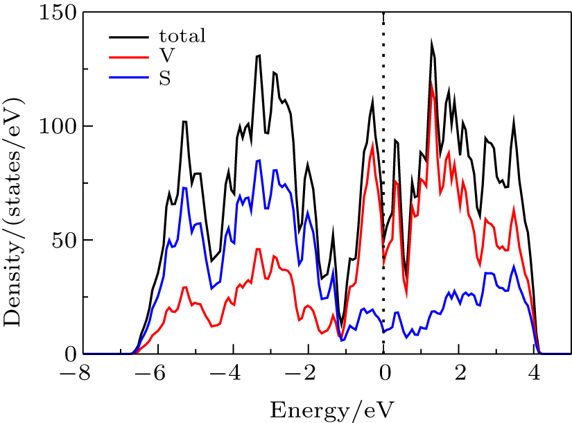
Fig. 1. HAADF-STEM images taken from different regions of a V₅S₈ single crystal. (a)–(c) HAADF-STEM images with different sizes. (d) Color-coded STEM image reveals clearly the V^I rectangular configuration (the brightest yellow dots).

Fig. 1. Structural and magnetic properties of V₅S₈ bulk single crystal. (a) HAADF-STEM image. Lower inset, a zoom-in image with the in-plane atomic model. Upper inset, a reduced FFT image. (b) The magnetic unit cell with the V^IS₆ octahedron. The blue arrows indicate the direction of the magnetic moments on V^I sites. (c) The molar magnetic susceptibility χ for B_⊥ ( B⊥ ab plane) and B_∥ (B ∥ ab plane). The inset shows the low temperature (T = 2 K) isothermal magnetization curves. (d) The inverse magnetic susceptibility 1/(χ – χ₀) for B_⊥. The blue dashed line is a linear fit of the Curie–Weiss law, which gives θ = 8.8 K, χ₀ = 0.01 cm³ ⋅ mol⁻¹, and μ_eff = 2.43μ_B per V^I.

Fig. 1. Calculated total (black lines) and species-projected density of states (V: red lines; S: blue lines) of V₅S₈ bulk. The dash line at the 0 eV represents the Fermi level.

Fig. 2. The atom-projected density of states (PDOS) of V^I (solid red curve), V^II (dashed blue curve), and V^III (dot-dashed green curve) in V₅S₈ bulk.

Fig. 2. Specific heat C of a 3.5 mg VSe₂ single crystal. VSe₂ displays no magnetic transition. At low temperatures, C/T is linearly dependent of T². A linear fit yields a Sommerfeld coefficient γ ∼ 11.5 mJ⋅K⁻² per mole of VSe₂ formula, shown in the inset.

Fig. 2. Specific heat. (a) The specific heat C as a function of temperature. The inset shows a C/T versus T² plot. The solid line is a linear fit, which yields γ = 74 mJ⋅K⁻²⋅mol⁻¹. (b) The low-T specific heat. C_e (dashed line) is the linear term γ T deduced from (a); the lattice contribution (dotted line), C_la = β T³, is inferred from the Debye model fitting; the magnetic term C_mag (dash-dot line) is extracted by the fitting to Eq. (1). The sum of all three contributions, that is, the fitting curve using Eq. (1) (the solid line) is in good agreement with the experimental data (red circles). (c) The non-lattice part of specific heat Δ C for three types of samples with different T_N. The dashed lines are the fits using Eq. (1) without β T³. The inset shows the fitting parameters as a function of T_N. (d) The relationship between the discontinuity of specific heat at T_N(δ C) and T_K/T_N.

Fig. 3. Temperature dependence of resistivity. (a) The temperature-dependent resistivity of three samples. The inset illustrates the high-T resistivity after subtracting the non-magnetic ρ of VSe₂ from that of V₅S₈. The dotted lines are the –ln T fits. (b) Fits of the low-T (T < 10 K) resistivity ρ/ρ(T = 50 K) for the three samples in (a). The dashed lines indicate the fits using Eq. (4), the fitting results are shown in the lower right. The A and Δ are in units of μΩ⋅cm⋅K⁻² and K, respectively. (c) Temperature dependent resistivity at different fields. (d), (e) The low-T resistivity ρ/ρ(T = 50 K) for sample A1 at different magnetic fields (B ⊥ ab plane). Dot-dashed lines are fits to Eq. (4). (e) The fitted gap of sample A1 as a function of field. The curves in (b)–(d) are vertically shifted for clarity.

Fig. 3. (a) Comparison of the temperature dependent resistivity ρ(T) between V₅S₈ and VSe₂. ρ versus T. VSe₂ displays a linear-T dependence, except for an anomaly at ∼ 90 K, which is due to a charge density wave transition. The dotted line is the baseline subtracted from the resistivity of V₅S₈ so as to highlight the contribution of the intercalation, Δ ρ. (b) Δ ρ as a function of temperature.

Fig. 4. Scaling of magnetoresistance for sample A1. (a) Magnetoresistance MR at various temperatures. The curves are vertically shifted for clarity. (b) Normalized resistivity versus B/(T + T^*), where T^* is a scaling parameter.

Fig. 4. Anomalous Hall effect and the carrier density of V₅S₈. (a) Hall resistivity ρ_xy (vertically shifted for clarity) at different temperatures. (b) Linear relation between the Hall coefficient R_H and the magnetic susceptibility χ above T_N. The blue line is a linear fit.

Fig. 5. Temperature-dependent thermopower S. S changes its sign at about 140 K and displays a negative minimum at 60 K.