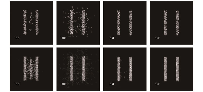
Fig. 1. Reconstructed images of two 200 nm stripes apart generated by different algorithms, density of the strip is 1μm-2 (above) and 51 μm-2 (below), respectively

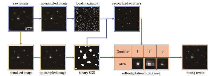
Fig. 2. Flowchart of SM algorithm, where the process of binary SNR generation, emitter identification and self-adaptation fitting algorithm are represented by yellow, blue and orange arrows, respectively

Fig. 3. Simulation data and algorithm comparison on simulation data. (a) Simulated images with different densities; (b) comparison of metrics of different algorithms; (c) localization error of different algorithms; (d) simulated reference image (ground truth,GT); (e) sectional intensity profiles and local magnification of reconstructed super-resolution images by different algorithms

Fig. 4. Algorithm comparison on experiment data. (a) rFRC maps of super-resolution images obtained from different algorithms; (b)‒(c) local magnification of super resolution images; (d) sectional intensity profile corresponding to white lines in Fig. 4(b)

Table 1. Comparison of super-resolution images recovered from different algorithms with ground truth image

Table 2. Quantitative resolution features of different algorithms given by rFRC

Table 3. Comparison of SE, ME and SM algorithms