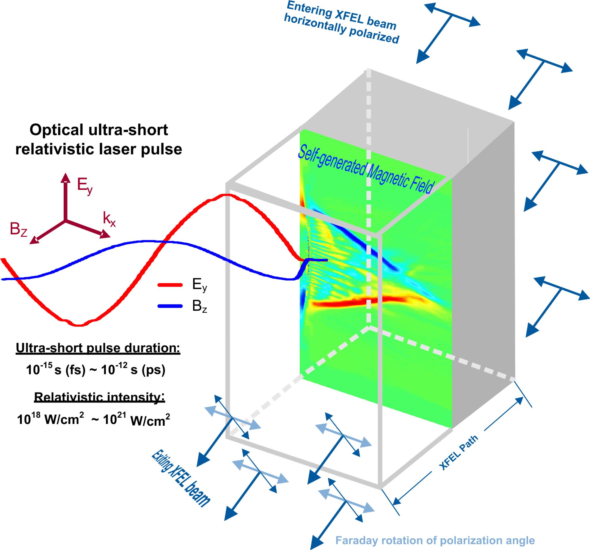
Fig. 1. An illustrated experimental setup of strong magnetic field generation by interaction of an ultra-short relativistic optical laser pulse with solid matter, probed by an XFEL via Faraday rotation.

Fig. 2. Two-dimensional spatial distributions of (a) longitudinal current density $j_{x}$, (b) transverse current density $j_{y}$, (c) total current density vector $\vec{j}$ and (d) magnetic field $B$ at the time $t=24~\text{fs}$ after laser peak intensity irradiating on the target. Throughout the whole text $t=0~\text{fs}$ is defined to be the reference time when the laser peak intensity irradiates on the front surface of the solid target. The black arrow shows the current direction. In the whole text, the physical and numerical parameters are similar to our previous work, as listed in Table 1^[9] and briefly introduced in Section 2. The difference will be highlighted in the figure captions. For this specific simulation, we assume the laser peak intensity $10^{20}~\text{W}/\text{cm}^{2}$ and exponential preplasma with scale length of $0.1~\unicode[STIX]{x03BC}\text{m}$ in front of the target. The target material is Cu with $20~\unicode[STIX]{x03BC}\text{m}$ thickness. This simulation uses the TF ionization model, which assumes local thermal equilibrium (LTE) condition.

Fig. 3. The spatial distributions of self-generated magnetic field in laser irradiated solid Cu target as the preplasma scale length varies from 0 to $0.4~\unicode[STIX]{x03BC}\text{m}$ at $t\approx 80~\text{fs}$. The thickness of the target is $2~\unicode[STIX]{x03BC}\text{m}$. All other simulation parameters are the same as Figure 2.

Fig. 4. The scaling of total laser absorption efficiency $\unicode[STIX]{x1D712}_{\text{total}}$ and maximum magnetic field by ponderomotive current and Weibel-like instability with the preplasma scale length.

Fig. 5. The spatial distributions of self-generated magnetic field in the cases of laser intensity and spot size at (a) $I_{0}=6.25\times 10^{18}~\text{W}/\text{cm}^{2}$, $R=8~\unicode[STIX]{x03BC}\text{m}$, (b) $I_{0}=2.5\times 10^{19}~\text{W}/\text{cm}^{2}$, $R=4~\unicode[STIX]{x03BC}\text{m}$ and (c) $I_{0}=1.0\times 10^{20}~\text{W}/\text{cm}^{2}$, $R=2~\unicode[STIX]{x03BC}\text{m}$ at $t\approx 80~\text{fs}$, respectively. The laser energy is fixed to ${\sim}0.2~\text{J}$. Instead of the LTE TF ionization model, the NLTE DI ionization model is used for these two specific simulations. The dependence of ionization model on magnetic field generation is investigated in our other work^[9]. The scale length of preplasma is $0.1~\unicode[STIX]{x03BC}\text{m}$ for these simulations. All other simulation parameters are the same as Figure 3.

Fig. 6. The spatial distributions of the self-generated interface magnetic field at $t\approx 80~\text{fs}$ (first row) and electron energy density at $t\approx -3~\text{fs}$ (second row) in layered target $\text{CH}_{2}$–Ti irradiated by laser pulse intensity $10^{19}~\text{W}/\text{cm}^{2}$ for different incident angles ranging from $0^{\circ }$ to $75^{\circ }$. Here we assume no preplasma in front of the target. The scale length of preplasma is $0~\unicode[STIX]{x03BC}\text{m}$ for these simulations. All other simulation parameters are the same as Figure 5.

Fig. 7. The spatial distributions of free electron density and self-generated magnetic field in a laser irradiated Cu target with $20~\unicode[STIX]{x03BC}\text{m}$ and $2~\unicode[STIX]{x03BC}\text{m}$ thicknesses at $t=24~\text{fs}$. $B_{z}^{\max }$ and $B_{z}^{\text{ave}}$ are the maximum and spatially averaged magnetic fields in the indicated regions. The scale length of preplasma is $0.1~\unicode[STIX]{x03BC}\text{m}$ for these simulations. All other simulation parameters are the same as Figure 2.

Fig. 8. The spatial distribution of magnetic field for (a) a $2~\unicode[STIX]{x03BC}\text{m}$ Ti single layer target and (b) a target with an additional $1~\unicode[STIX]{x03BC}\text{m}~\text{CH}_{2}$ layer in the front at $t\approx 80~\text{fs}$, respectively. NLTE DI ionization model is used here. The scale length of preplasma is $0.1~\unicode[STIX]{x03BC}\text{m}$ for these simulations. All other simulation parameters are the same as Figure 7.

Fig. 9. The spatial distribution of magnetic field for two layers target (a) $\text{CH}_{2}$–Al, (b) $\text{CH}_{2}$–Ti and (c) $\text{CH}_{2}$–Au without preplasma at $t\approx 80~\text{fs}$, respectively. Here we assume the peak laser intensity $10^{19}~\text{W}/\text{cm}^{2}$ and no preplasma in front of the target. All other simulation parameters are the same as Figure 8(b).