Propagation dynamics of ring Airy Gaussian beams with cosine modulated optical vortices

Feili Wang; Cibo Lou; Yi Liang

doi:10.3788/COL201816.110502

Abstract

We numerically investigate the propagation properties of ring Airy Gaussian beams (RAGBs) with cosine modulated optical vortices (CMOV). In comparison to the common RAGBs without any modulation, the dynamic propagation of RAGBs with CMOV exhibits a unique feature: the rings of RAGBs with CMOV will gradually shrink into several main lobes with the increase of the propagation distance. The number of lobes and the peak intensity of each lobe are determined by the factors of cosine modulated function. By designing the initial phase, we can easily change the transversal location of the peak intensity. Our results may find potential applications in optical manipulations.

In the past a few years, circular Airy beams (CABs) have attracted a lot of attention due to their abrupt autofocusing property, which brings about many potential applications in optical micromanipulations^[1–5]. For realizing a stable and easy micromanipulation, optical beams should generate large optical trapping forces, which are related to their intensity gradients. To further enhance the intensity gradient of CABs at the focal plane, introducing optical vortices to the beam structures is proposed, which will create hollow intensity profiles at the focal plane to generate stronger optical trapping^[6–12]. Recently, several related works have proposed and investigated such beams^[13–18].

Here, by imposing a cosine modulated optical vortex (CMOV) onto a ring Airy Gaussian beam (RAGB), we design a CAB with a special beam profile for generating an interesting intensity gradient distribution for optical trapping applications. The propagation dynamics of the new beams are studied by employing numerical simulations. Our results show that, the same as CABs, the beams still have some rings at the beginning. However, as the propagation distance increases, these rings will shrink gradually and evolve into several main lobes. The positions, numbers, and peak intensities of the main lobes could be easily controlled by the factors of the cosine modulated function. Especially, by changing the factors of modulated function, we can easily adjust the focal intensity and focal length of the autofocus RAGB with CMOV. Moreover, we find that the modulated initial phase will determine the peak intensity position of each main lobe at the transverse plane.

Theoretically, the electric field of an initial RAGB with CMOV can be expressed as $u (r, φ, z = 0) = A_{0} A i (\frac{r_{0 -} r}{b w}) \exp (a \frac{r_{0 -} r}{b w}) \exp [- \frac{{(r_{0} - r)}^{2}}{w^{2}}] [r^{l} e^{i l φ (θ)}],$ (1)where $A_{0}$ is the amplitude of the input electric field, $A i (\cdot)$ represents the Airy function, $r_{0}$ is the beginning radius of the main Airy ring, $a$ is an exponential decay factor, $b$ is a scaling factor, $w$ is a radial scale, $r = \sqrt{x^{2} + y^{2}}$ is the radial coordinate, $x$ and $y$ are the transversal coordinates of $u$ , $l$ represents the topological charge of the optical vortex, $θ = arctan (y / x)$ is an azimuthal angle, and $φ (θ)$ is introduced as the cosine modulated function, which can be expressed as $φ (θ) = C_{0} \cos (m θ) \cos (n θ + φ_{0}),$ (2)where $C_{0}$ is a constant, which can adjust the magnitude of the modulation, and $m$ and $n$ are the numbers of phase folds of the first and second cosine function, respectively. $φ_{0}$ is the initial modulated phase of its second cosine function.

Sign up for Chinese Optics Letters TOC. Get the latest issue of Chinese Optics Letters delivered right to you！Sign up now

Within the framework of the paraxial approximation, by using the electric field of RAGB described by Eq. (1) as an input, we can observe the propagation of RAGBs through simulating the diffraction equation with the split-step Fourier method^[19–21]: $\frac{1}{2 k} (\frac{\partial^{2}}{\partial x^{2}} + \frac{\partial^{2}}{\partial y^{2}}) u + i \frac{\partial u}{\partial z} = 0,$ (3)where $u$ is the amplitude of the electric field, $k = 2 π / λ$ is the wave number in free space, $λ$ is the wavelength of the incident light, and $z$ is the longitudinal propagation distance.

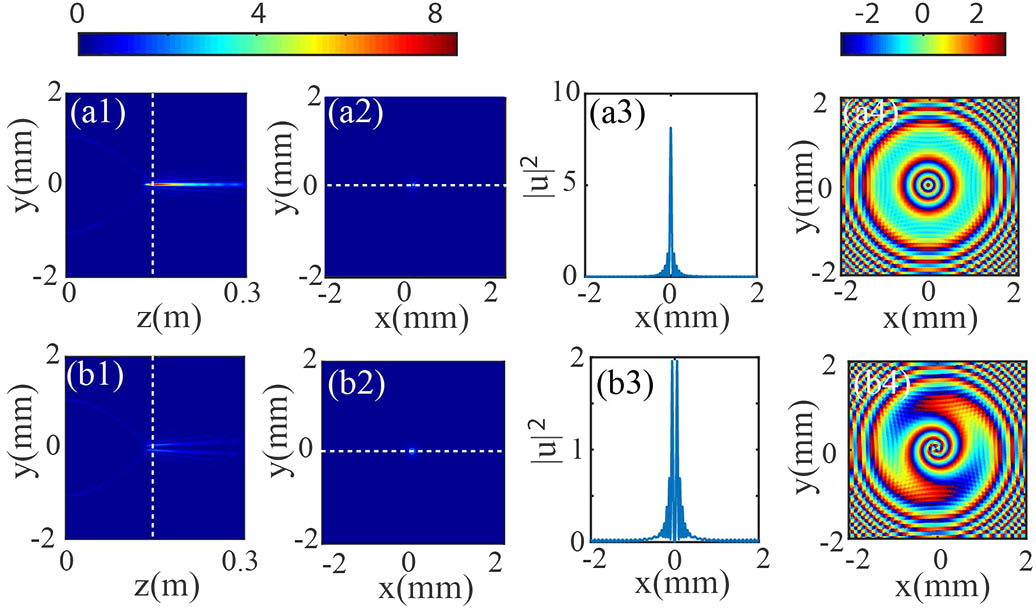
First, we use the following simulation parameters: $r_{0} = 1 mm$ , $w = 0.5 mm$ , $a = 0.05$ , $b = 0.1$ , and the wavelength $λ = 1064 nm$ . In order to highlight the effect of the modulated vortex structure on the propagation dynamics of RAGBs in free space, the topological charge of the optical vortex $l$ is set to be 2. When $C_{0} = 0$ , the beam is a common RAGB, as shown in Figs. 1(a1)–1(a4). Clearly, it is a typical abruptly autofocusing beam, which is cylindrically symmetric and able to abruptly autofocus during the propagation. Figures 1(b1)–1(b4) present the propagation of an RAGB with a conventional vortex [ $φ (θ) = θ$ ]. As mentioned in Ref. [6], because of the huge intensity gradient produced by the hollow core at the focus plane, this kind of beam can exhibit a strong micro particles trapping ability. When $C_{0} = 1$ , for different modulated vortex structures, the beams will have different propagation behaviors.

Figure 1.(a1) The side-view propagation of a common RAG beam; (a2) the intensity profile at the focus plane marked by the dashed line in (a1); (a3) the distribution of ${| u |}^{2}$ marked by the dashed line in (a2); (a4) the phase pattern of the common RAG beam at the focus plane; (b1)–(b4) are the corresponding properties of the RAGB.

When $m = 0$ , $φ (θ) = C_{0} \cos (n θ + φ_{0})$ . For this modulated vortex structure, we first adopt $C_{0} = 1$ , $n = 3$ , and $φ_{0} = 0$ . Figure 2 shows the intensity and phase distributions of the RAGB with this CMOV as the propagation distance changes. In comparison with the common RAGBs shown in Fig. 1, the rings of the RAGB split into three main lobes and then shrink into many smaller lobes with the distance increasing. Notice that the beams show a triangular symmetry. Figures 2(b1)–2(b5) are the corresponding phase patterns of Figs. 2(a1)–2(a5). We can see that the phase pattern formats three main pits in the phase spots, and the three main phase pits can remain stable once the pits have been formed. While for the intensity distributions, as shown in Figs. 2(a1)–2(a5), we can see that the borders of phase pits are the angles where the three main lobes appear in the polar coordinate system. Moreover, the borders of phase pits are the angle of maxima value of the initial phase at the transverse plane.

Figure 2.Intensity and phase patterns of RAGB with CMOV with the parameters $C_{0} = 1, m = 0, n = 3$ , and $φ_{0} = 0$ during propagation. (a1)–(a5) The intensity distributions of the RAGB with CMOV for various propagation distances $z = 0 m$ , 0.04 m, 0.08 m, 0.12 m, 0.16 m, respectively; (b1)–(b5) are the corresponding phase distributions of (a1)–(a5).

In fact, the factor $n$ determines the number of the final main lobes of the beams after evolution. For example, Fig. 3 presents the intensity distributions and phase distributions of the RAGB with CMOV for different factors $n = 0, 1, 2, 3, 4$ . It is evident that the RAGB with CMOV will have 0, 1, 2, 3, 4 main lobes at the position $z = 0.12 m$ . Meanwhile, it is also found that the initial phase $φ_{0}$ affects the distributed angle of the main branches. When we change the $φ_{0}$ , the main lobes, including intensity and phase patterns, rotate $φ_{0} / n$ along the clockwise direction (Fig. 4).

Figure 3.Intensity and phase patterns of RAGB with CMOV for various $n$ at the distance $z = 0.12 m$ when $C_{0} = 1, m = 0$ , and $φ_{0} = 0$ . (a1)–(a5) are the beam spots for $n = 0, 1, 2, 3, 4$ , respectively; (b1)–(b5) are the corresponding phase distributions of (a1)–(a5).

Figure 4.Intensity and phase patterns of RAGB with CMOV for various $φ_{0}$ at the distance $z = 0.12 m$ when $C_{0} = 1, m = 0$ , and $n = 3$ . (a1)–(a5) are the beam spots for $φ_{0} = 0, \frac{π}{2}, π, \frac{3 π}{2}, 2 π$ , respectively; (b1)–(b5) are the corresponding phase distributions of (a1)–(a5).

Figure 5 depicts the abruptly autofocusing property of RAGBs with $φ (θ) = C_{0} \cos (n θ + φ_{0})$ . Here, we assume the maximum intensities at the initial plane and different propagation distances are $I_{0}$ and $I_{m}$ . In order to clearly compare the peak intensities with different $n$ , we use the ratio of $I_{m}$ to $I_{0}$ to analyze their propagation. Clearly, at the beginning, the peak intensities stay low before the focus plane. Then, they rapidly increase at the focal point. It should be noted that, the peak intensities at the focal plane with different $n$ are different. When the factor $n = 0$ (the common RAGB), the peak intensity can increase by 27.5 times at the focal point. However, when the factor $n = 1, 2, 3, 4$ , the peak intensities only increase by about 27.3, 9.4, 8.2, 5.9 times, i.e., as $n$ increases, the enhancing of the peak intensities at focal point will decrease [Fig. 5(b)] even though their autofocusing positions are nearly the same, which are located at about $z = 0.15 m$ .

Figure 5.(a) The peak intensity distributions of the RAGB with CMOV during propagation for $m = 0$ , $n = 0, 1, 2, 3, 4$ , respectively; (b) the max peak intensities of (a) for various $n$ .

Next, we shall study the propagation characteristics of RAGBs with CMOV when $φ (θ) = C_{0} \cos (m θ) \cos (n θ + φ_{0})$ . Here, we choose the factor $C_{0} = 1, m = 1$ , and the factor $n = 0, 1, 2, 3, 4$ to perform the simulation, as shown in Figs. 6–10. Figure 6 shows the intensity and phase distributions of the RAGB with CMOV with the factor $n = 1$ at the propagation distance $z$ of 0, 0.04, 0.08, 0.12, and 0.16 m. From Fig. 6, we can see that the intensity distributions during propagation have similar characteristics to that of Fig. 2. The spots first split into three main lobes and then shrink as the propagation distance increases. The modulated phase spots also form several main pits gradually with the distance increasing.

Figure 6.Intensity and phase patterns of the RAGB with CMOV with the parameters $m = 1, n = 2$ , and $φ_{0} = 0$ during propagation. (a1)–(a5) The intensity distributions of the RAGB with CMOV for various propagation distances $z = 0 m$ , 0.04 m, 0.08 m, 0.12 m, 0.16 m, respectively; (b1)–(b5) are the corresponding phase distributions of (a1)–(a5).

However, the peak intensities of three main branches are different. In Fig. 6(a4), the right branch (A) has greater peak intensity than the other two (B and C). Figure 7 shows the initial modulation phase distribution at $z = 0 m$ and the peak intensity distribution at $z = 0.12 m$ along with the spiral phase $θ$ at different $m$ and $n$ . In Fig. 7(a), each maximum value of the initial phase is equal, and the peak intensity of each branch is equal. In Fig. 7(b), the branch that has maximum phase value will show much greater peak intensity, i.e., the initial modulation phase will affect the peak intensities of the branches at the focal point. It should be noted that, in this case, the initial phase $φ_{0}$ still affects the distributed angle of the main lobes, the same as Fig. 4 (Fig. 8). Moreover, the initial phase maximum will decide where the lobe with maximum intensity appears, as shown in Fig. 8.

Figure 7.The modulation phase distributions and the intensity distributions at $z = 0 m$ and $z = 0.12 m$ versus the spiral phase $θ$ when $C_{0} = 1, φ_{0} = 0$ for different factors $m$ and $n$ . (a) $m = 0, n = 3$ ; (b) $m = 1, n = 2$ .

Figure 8.Intensity and phase patterns of RAGB with CMOV for various $φ_{0}$ at the distance $z = 0.12 m$ when $C_{0} = 1, m = 1$ , and $n = 2$ . (a1)–(a5) The beam spots for $φ_{0} = 0, \frac{π}{2}, π, \frac{3 π}{2}, 2 π$ , respectively; (b1)–(b5) are the corresponding phase distributions of (a1)–(a5).

Figure 9 shows the intensity and phase distributions of RAGB with CMOV at the position $z = 0.12 m$ with the factor $m = 1$ , $n = 0, 1, 2, 3, 4$ , respectively. Our results show that the number of final lobes at the focal point equals the sum of $m$ and $n$ .

Figure 9.Intensity and phase patterns of RAGB with CMOV for various $n$ at the distance $z = 0.12 m$ when $C_{0} = 1, m = 1$ , and $φ_{0} = 0$ . (a1)–(a5) are the beam spots for $n = 0, 1, 2, 3, 4$ , respectively; (b1)–(b5) are the corresponding phase distributions of (a1)–(a5).

Figure 10(a) presents the abruptly autofocusing properties of RAGB with CMOV in this case. One can find that the modulated phase factor $m$ will not change the autofocusing position. Furthermore, for $m = 1$ , $n = 0, 1, 2, 3, 4$ , the peak intensity can increase by about 26.9, 15.8, 16.0, 11.2, 12.2 times that of initial plane at the focal plane. Figure 10(b) indicates it more clearly. As the value of the factor $n$ increases, the enhancement of the peak intensity at the focus point first goes down, then goes up slightly, and then goes down again. Especially, the peak intensity is basically the same for the factor $n = 1, 2$ . When $m = 2$ , the beam spots are clearly shown in Fig. 11. The peak intensity at the focal plane can increase 9.4, 16.1, 16.0, 16.1, 10.1 times, respectively (Fig. 12). Particularly, the enhancement of the peak intensity at the focus point first goes up and then goes down. It is found that the peak intensity is almost the same for the factor $n = 1, 2, 3$ . This indicates that the peak intensity at the focal point and the transverse location of the peak intensity during propagation can be controlled by choosing appropriate factors.

Figure 10.(a) Peak intensity distributions of the RAGB with CMOV during propagation for $m = 1$ , $n = 0, 1, 2, 3, 4$ , respectively; (b) the max peak intensities of (a) for various $n$ .

Figure 11.Intensity and phase patterns of RAGB with CMOV for various $n$ at the distance $z = 0.12 m$ when $C_{0} = 1, m = 2$ , and $φ_{0} = 0$ . (a1)–(a5) are the beam spots for $n = 0, 1, 2, 3, 4$ , respectively; (b1)–(b5) are the corresponding phase distributions of (a1)–(a5).

Figure 12.(a) Peak intensity distributions of the RAGB with CMOV during propagation for $m = 2$ , $n = 0, 1, 2, 3, 4$ , respectively; (b) the max peak intensity of (a) for various $n$ .

In summary, we have studied the propagation properties of RAGBs with CMOV. By changing the factor of the cosine modulated function, the rings of RAGB with CMOV shrink into several main lobes with the increase of propagation distance. It is also found that the number of the main lobes equals the value of $m$ plus $n$ . The initial phase $φ_{0}$ will change the distributed angle and the peak intensity of the main lobes, which means that we could easily control the distribution and intensity of each lobe. By adjusting the cosine modulated function factors $m$ , $n$ , and $φ_{0}$ , we can realize a convenient light control. For example, if we want to manipulate several micro particles at the same time, we can design an appropriate number of main lobes to trap each particle^[22]. Moreover, combined with a radially or circularly polarized beam, we may enhance the trapping rate and also rotate each particle as a optical needle^[23]. Our results may find many potential applications in optical tweezers, which is valuable in the biological field.