Simple optical method for small angular displacement measurement based on the astigmatic effect

Jinggao Zheng; Qun Wei; Linyao Yu; Mingda Ge; Tianyi Zhang

doi:10.3788/COL201614.030801

Abstract

We propose a novel small-angle measuring optical method based on the astigmatic effect of two orthogonally placed cylindrical lenses. According to the one-to-one correspondence between the laser spot shape and the angle, the angle is determined. We theoretically analyze the measuring range and demonstrate that a longer distance between the rotating axis and the optical axis leads to a smaller measuring range, but better sensitivity. Also, an associated experimental system is established and a measuring range of 0.94 mrad (cubic fit

r = 0.9993

) as well as a good linear range of 0.37 mrad (linear fit

r = 0.9994

) with a resolution of 8 μrad is achieved.

Small angular displacement measuring techniques have been widely used in modern engineering and scientific research, including the precision alignment of mechanical systems, the calibration of machine tools, coordinate measuring machines, and so on^[1,2]. Among them, optical systems are one of the most often used techniques, particularly when contact with the sample should be avoided and high precision is needed^[3,4]. There are mainly two kinds of optical methods adopted for measuring the angular displacement. One is based on interferometry^[5–8], and the other one is based on the optical autocollimator system^[9–11]. As an extension of the linear displacement measurement using interferometry, the interferometric angular displacement measurement is also implemented by counting the changes in interference fringes due to the variations of the optical path difference between the reference and sample arms^[7]. Therefore, by use of this angular displacement measurement, a high resolution can be achieved. However, the interferometric techniques not only consist of expensive and complicated devices, but also require highly stable environment. The system of the optical autocollimator utilizes a beam of collimated light on a flat mirror, and the back-reflected light is focused by an objective lens. Then, using the correspondence between the position of the spot in the focal plane of the lens and the rotated angle of the mirror, the angle is determined^[11]. Optical autocollimators do not suffer from complex setups or stringent condition requirements. Nevertheless, using this technique, one can also achieve high sensitivity and high accuracy. In recent years, several new small-angle measuring systems have been established based on total internal reflection^[12,13], parallel interference patterns^[14], prism^[15], fringe analysis^[16], and birefringence^[17], meeting the needs of different applications.

In this Letter, without using the aforementioned techniques, we propose a simple small-angle measuring optical method based on the astigmatic effect^[18–21]. Here, the astigmatic effect results from two perpendicularly placed cylindrical lenses (CLs). Also, a corresponding experiment is carried out, and our results demonstrate the capability of this non-contact small-angle measuring astigmatic method to be applied to the fields of metrology, manufacturing, and scientific research.

Like the interferometric angle measuring method, which can be regarded as a derivative of the linear displacement measuring technique using interferometry^[7], our method is an extension of linear displacement measurement based on the astigmatic effect. Therefore, to better understand the principle of our method, the linear displacement measuring astigmatic method is briefly introduced first.

Sign up for Chinese Optics Letters TOC. Get the latest issue of Chinese Optics Letters delivered right to you！Sign up now

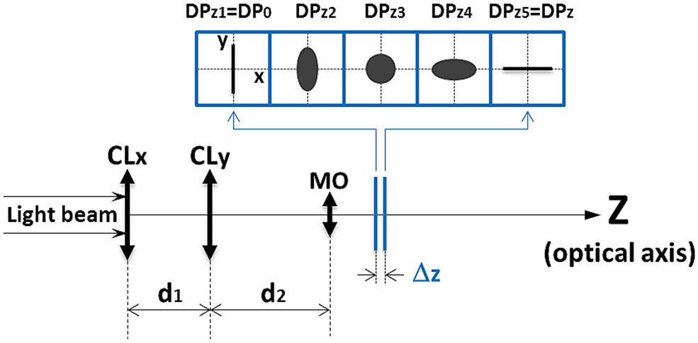
The schematic diagram of linear displacement measurement using the astigmatic effect is shown in Fig. 1^[18]. The system is made up of two perpendicularly placed CLs and a microscope objective (MO). Assuming that the optical axis is the $z$ -axis, CLx in Fig. 1 is a CL that has positive optical power only in the $x$ direction, while CLy is a CL that has optical power only in the $y$ direction. The two CLs are separated by a distance $d_{1}$ , and the distance between CLy and the MO is $d_{2}$ . For the real experimental system, because the lenses are not perfectly thin lenses, $d_{1}$ is in fact the distance between the two corresponding rear principle planes of CLx and CLy, while $d_{2}$ is the distance between the two corresponding rear principle planes of the CLy and MO. The two crossed CLs generate the astigmatic effect, while the MO can shorten the measuring range of the linear displacement measuring system to several microns, achieving a high sensitivity.

Figure 1.Schematic diagram of linear displacement measurement based on the astigmatic effect. The shape of the light spot is changed, as the DP varies its axial displacement along the optical axis ( $z$ -axis).

For this system, when the detection plane (DP) varies its axial displacement within a specified range $Δ z$ from $z_{1}$ (0 for relative displacement) to $z_{5}$ ( $z$ for relative displacement), the shape of the light spot affected by the two crossed CLs is changed from a vertical line along the $y$ -axis to its orthogonal horizontal line along the $x$ -axis. In other words, the shape changing of the light spot results from the different optical paths that light travels along on the optical axis. Using this one-to-one correspondence, the linear displacement measurement is realized and the measuring range can be considered as the distance $Δ z$ between ${DP}_{z 1}$ and ${DP}_{z 5}$ . Also, because the smaller $Δ z$ is, the more rapidly the shape of light spot changes from the vertical line to the horizontal line, the sensitivity of this linear displacement measuring astigmatic system is inversely proportional to $Δ z$ . Thus, to achieve a high measuring sensitivity, $Δ z$ should be minimized at the cost of shortening the measuring range.

The expression of $Δ z$ is $Δ z (d_{1}, d_{2}, f_{MO}, f_{x}, f_{y}) = \frac{d_{1} f_{MO}^{2}}{(f_{x} + f_{MO} - d_{1} - d_{2}) (f_{y} + f_{MO} - d_{2})},$ (1)where $f_{MO}$ , $f_{x}$ , and $f_{y}$ are the focal lengths of the MO, CLx, and CLy, respectively. It can be seen from Eq. (1) that smaller $f_{MO} / d_{1} / d_{2}$ or longer $f_{x} / f_{y}$ lead to smaller $Δ z$ and a higher measuring sensitivity. Additionally, if the incident light beam has a circular shape, the light spots on the DPs have elliptical shapes between the two orthogonal lines, as shown in Fig. 1. Moreover, it can be readily seen from Fig. 1 that the $x$ - and $y$ -axes are the two symmetrical axes of the laser spots.

The aforementioned optical path differences between the DPs can be also realized by rotating the DP about an axis some distance (not zero) away from the optical axis of the CLs. Figure 2 illustrates this effect.

Figure 2.Schematic diagram of the linear relationship between the axial translation along the optical axis ( $z$ -axis) and rotation about an axis (along $x$ -axis) a specified distance $L$ away from the $z$ -axis.

As shown in Fig. 2, ${DP}_{θ}$ ( $θ$ for relative angle) is the DP obtained by rotating the ${DP}_{0}$ (0 for relative angle) an angle of $θ$ about an axis (along the $x$ -axis) a specified distance $L$ away from the optical axis ( $z$ -axis). In this circumstance, the light reaching the ${DP}_{θ}$ travels a longer optical path than that reaching the ${DP}_{0}$ . The optical path difference $Δ z$ can be derived as follows: $Δ z = L \times \tan (Δ_{θ}),$ (2)If the rotated angle $θ$ is small so that $\tan (Δ_{θ})$ almost equals the value of $Δ_{θ}$ , the expression of $Δ z$ can be written as a linear form: $Δ z = L \times Δ_{θ} .$ (3)Therefore, using this linear relationship between $Δ z$ and $Δ_{θ}$ , one can also achieve the shape changes from a line to its orthogonal counterpart by rotating the DP from ${DP}_{0}$ to ${DP}_{θ}$ . In fact, because $Δ z$ is usually in the order of microns and the value of $L$ is in the order of millimeters, $Δ_{θ}$ can be easily made in order of sub-milliradians, which is much smaller than 1°. Then, the difference between $\tan (Δ_{θ})$ and $Δ_{θ}$ is even smaller than 1 nanoradians. This difference is about 3 or 4 orders of magnitude lower than the resolution of our angle measuring method, which is in order of microradians, and hence $\tan (Δ_{θ})$ certainly can be replaced with $Δ_{θ}$ to obtain the linear relationship between $Δ z$ and $Δ_{θ}$ , as shown in Eq. (3).

Figure 3 shows one typical schematic diagram of the angle measuring astigmatic method. In this diagram, when the rotated angle is 0°, the corresponding shape of the laser spot on the DP is a line along the $y$ -axis. If the rotated angle is kept at 0°, by adjusting the axial position of the DP within the axial measuring range $Δ z$ shown in Fig. 1, one can also obtain any other shapes of the laser spot. Therefore, the rotated angle of 0° can correspond to any one of the laser spot shapes from a line along the $y$ -axis to the orthogonal counterparts shown in Figs. 1 and 3. Thus, not to affect the angle measurement, once the axial position of the DP has been adjusted at the beginning prior to the angle measurement, it should be kept unchanged throughout the experiment.

Figure 3.Schematic diagram of small-angle measurement based on astigmatic effect. The shape of the light spot is changed, as the DP is rotated about an axis a distance $L$ away from the optical axis ( $z$ -axis).

Also, as the linear displacement measurement, the smaller the value of $Δ_{θ}$ , the more rapidly the shape of the light spot changes from the vertical line to the horizontal line, so the sensitivity of this small-angle measuring astigmatic system is inversely proportional to $Δ_{θ}$ . Thus, to achieve a high angle measuring sensitivity, $Δ_{θ}$ should be minimized. Using Eqs. (1) and (3), the expression of $Δ_{θ}$ can be readily derived as follows: $Δ_{θ} (L, d_{1}, d_{2}, f_{MO}, f_{x}, f_{y}) = \frac{Δ z}{L} = \frac{d_{1} f_{MO}^{2}}{L (f_{x} + f_{MO} - d_{1} - d_{2}) (f_{y} + f_{MO} - d_{2})} .$ (4)Compared with the linear displacement measurement, there is one more parameter, $L$ , affecting the measuring range in the angular displacement measurement. As the distance $L$ between the rotating axis and the optical axis becomes larger, the angle measuring range gets smaller, and hence the sensitivity is made higher.

To show the feasibility of our angular displacement measuring method, a corresponding experiment is carried out. The schematic diagram of the experimental setup is shown in Fig. 4. The light source is a He–Ne laser with a wavelength of 632.8 nm (HN050 L, Thorlabs). Not to saturate the CCD (CS8620, Teli), an attenuator is placed after the light source. Furthermore, to make the laser spot as uniform as possible before the laser beam reaches CLx, the laser beam transmits through a beam expander. A beam splitter (BS) is utilized to generate a distorted laser spot on one side and detect the reflected and magnified laser spot on another side. After passing through the BS, the shape of the laser spot is changed due to the astigmatic effect generated by two identical but perpendicularly placed plano-convex CLs (CLx and CLy) whose focal lengths are both 150 mm. The distance between the two corresponding rear principle planes of CLx and CLy (or $d_{1}$ in Fig. 3) is adjusted to be 3 mm. A $65 \times$ MO with the focal length of 4 mm is inserted after CLy to achieve a high sensitivity. Also, due to the thicknesses of MO and its holder, the distance between the two corresponding rear principle planes of the CLy and MO (or $d_{2}$ in Fig. 3) is 50 mm. The laser spot focused by the MO is too small to directly image on the CCD, so a mirror is located at the DP and the light rays are reflected toward the imaging lens (IL), by which the laser spot can be magnified. The mirror is controlled by a motorized rotation stage to implement the angle change with the step of 0.003°, and a translation stage is employed to separate the rotating axis 5 mm away from the optical axis. The reflected light rays go back to the BS via the MO and the two CLs. Then the laser spot is magnified and imaged on the CCD by the IL with a focal length of 500 mm. According to Eq. (4), the theoretical measuring range is calculated to be about 0.05°, or 0.9 mrad.

Figure 4.Schematic diagram of the experimental setup. BE, beam expander.

The laser spot images corresponding to different rotated angles are shown in Fig. 5. The angle interval between the two adjacent images in Fig. 5 is 0.009°. It can be readily noticed from Fig. 5(a) that the two symmetrical axes (previously the $y$ - and $x$ -axes) of the laser spot are not in the vertical and horizontal directions, but one symmetrical axis (SA1, previously the $y$ -axis) is in the direction of 45° and the other one (SA2, previously the $x$ -axis) is in the direction of 135°. This is because we have done the image processing of simple rotation to the raw CCD images to simplify another image processing, which is used to extract the rotated angles from the laser spot images. Also, from Figs. 5(a)–5(h), the energy of the laser spot first distributed mainly in the direction of 45°. But then, as the rotated angle of the mirror changes, there is more and more energy distributed in the other orthogonal direction. As a result, the shape of the laser spot is changed when the mirror is rotated. Using this one-to-one correspondence between the shape of the laser spot and the rotated angle, the angle is determined. Additionally, it should be pointed out that the laser spots do not form ideal lines or elliptical shapes in Fig. 5. This is because the laser spot is not only affected by the astigmatism, but it is also affected by spherical or higher-order aberrations that result from the imperfect optical elements, including the two CLs, MO, and IL, etc.

Figure 5.Laser spot images corresponding to different relative rotated angles of (a) 0°, (b) 0.009°, (c) 0.018°, (d) 0.027°, (e) 0.036°, (f) 0.045°, (g) 0.054°, and (h) 0.063°. SA1 and SA2 in (a) are two symmetrical axes of the laser spot. The numbers 1 to 4 in (h) designate four segmented quadrants.

To quantify the one-to-one correspondence and to extract the value of the angle from the laser spot image, a very simple image processing is utilized that the astigmatic focusing error signal (FES) of each image is calculated with four-quadrant difference processing^[18,19]. The FES is defined as $FES = \frac{- E_{1} + E_{2} - E_{3} + E_{4}}{E_{1} + E_{2} + E_{3} + E_{4}},$ (5)where $E_{i}$ is the total energy of the laser spot in the $i$ th quadrant. To use this algorithm, each image of the laser spot is segmented into four quadrants and the centroid of the laser spot is used as the coordinate origin, as demonstrated in Fig. 5(h).

The quantitative relationship between the FES and angle is illustrated in Fig. 6(a). The curve has the expected S-shape. As mentioned previously, a smaller measuring range indicates that the laser spot changes its shape more rapidly from a line to its orthogonal counterpart. Thus, better sensitivity can be obtained with a smaller measuring range, while a larger correlation coefficient $r$ of the fitted line shows a higher fitting precision. Moreover, different angles that have the same corresponding values of FES cannot be distinguished from each other. Therefore, when calculating the measuring range, only the monotonous zone of the S-curve should be taken into account. In Fig. 6(a), the measuring range is 0.054° (from 0.009° to 0.063°), or 0.94 mrad. If the cubic polynomial fit is applied to this measuring range, we can yield the following fitted equation: $y_{1} = - 410826.63 x_{1}^{3} + 44588.25 x_{1}^{2} - 341.99 x_{1} - 21.34,$ (6)and the correlation coefficient $r = 0.9993$ .

Figure 6.(a) The quantitative relationship between the FES and rotated angle of the mirror. (b) $Δ_{1}$ : the angle differences between the cubic fit and experimental data that have the same values of FES; $Δ_{2}$ : the angle differences between the linear fit and experimental data that have the same values of FES.

While the linear fit is applied to angles within the range of 0.021° (from 0.024° to 0.045°), or 0.37 mrad, we obtain the fitted equation $y_{2} = 1170.47 x_{2} - 37.55,$ (7)and the correlation coefficient $r = 0.9994$ .

Therefore, our data show good coincidence with the cubic fitted line ( $r = 0.9993$ ) within the range of 0.054° (0.94 mrad), and $Δ_{1}$ in Fig. 6(b) shows the angle differences between the cubic fitted line and experimental data that have the same values of FES. Also, our data show excellent linearity ( $r = 0.9994$ ) within the range of 0.021° (0.37 mrad), and $Δ_{2}$ in Fig. 6(b) shows the angle differences between the linear fitted line and the experimental data that have the same values of FES. If the experimental data show this high linear correlation, one-tenth to one-fifth of the step can be recognized as a reasonable resolution^[18], so the resolution of our system is about 0.00045° (8 μrad), according to the step of 0.003°. This reasonability can be seen from $Δ_{2}$ that the biggest value in $Δ_{2}$ is 0.00040°, which is even smaller than 0.00045° (reasonable resolution calculated above), and the root mean square value of the angle differences in $Δ_{2}$ is only 0.00024°. This resolution is comparable to those of commercially available products^[22] whose resolutions are also in the order of microradians, and it can be further improved when using a four-quadrant detector instead of a CCD. This is because the four-quadrant detector has a lower noise level than the CCD. Furthermore, since our method is a derivative of the linear displacement measuring technique based on CLs, our method has the property of strong noise immunity^[18] as well, and the noise that affects the resolution also comes from the stability of the system, data acquisition and processing, environment disturbances, and positioning errors of the translation and rotation stages. Moreover, because the sensitivity gets higher at the cost of shortening the measuring range, one should make a trade-off between the sensitivity and the measuring range according to the requirements.

In addition, it can be noticed from Fig. 6(a) and the fitting analysis above that the detectable angles do not begin from 0° in both fits, and the starting value of angle (0.024°) in the linear fit is even larger than the detectable linear range (0.021°), both of which are bad for a practical application. These points result from the fact that in order to fully demonstrate the S-shape of the FES curve, at the beginning of our experiment before the angle measurement, we have chosen the mirror’s axial position, which is out of the axial displacement measuring range in Fig. 1. As a result, the value of FES corresponding to the rotated angle of 0° is not in the cubic fit range shown in Fig. 6(a), and the detectable angles do not begin from 0° for both fitting ranges. However, as analyzed previously, by adjusting the axial position of the mirror prior to the angle measurement with a translation stage, one can always make the detectable beginning angle 0°. Therefore, whether the detectable angle begins from 0° or not depends on the initially fixed axial position of the mirror. In detail, for the cubic fit, by adjusting the axial position of the mirror, the value of FES corresponding to the rotated angle of 0° can be made equal to the starting value of FES in the cubic fit in Fig. 6(a). For the linear fit, the value of FES corresponding to the rotated angle of 0° can be made equal to the starting value of FES in the linear fit in Fig. 6(a). By using these adjustments at the very beginning of the experiment, the detectable rotated angles can begin from 0°, and hence, the starting values of the angles are also within the detectable ranges for both fits.

In conclusion, a novel optical method for small angular displacement measurement is proposed based on the astigmatic effect, which is generated by two orthogonally placed CLs. For this system, the laser spot has different shapes when the DP is rotated about an axis some distance away from the optical axis. The angle is then determined according to one-to-one correspondence. Also, the measuring range and sensitivity of the method is theoretically analyzed, and we demonstrate that a longer distance between the rotating axis and optical axis leads to a smaller measuring range, but better sensitivity. Further, in our experiment, the measuring range of 0.94 mrad (cubic fit $r = 0.9993$ ) as well as the good linear range of 0.37 mrad (linear fit $r = 0.9994$ ) with the resolution of 8 μrad is achieved. Our results reveal the potential of this simple astigmatic method as a non-contact small-angle measuring tool that is useful in industrial and scientific research.

References

[1] G. Hussain, M. Ikram. Opt. Lett., 33, 2419(2008).

[2] G. Hussain, M. Ikram. Appl. Opt., 49, 1025(2010).

[3] G. Hussain, M. Ikram. Opt. Lett., 29, 1930(2004).

[4] S. Z. Tang, Z. Wang, J. M. Gao, J. J. Guo. Rev. Sci. Instrum., 85, 045110(2014).

[5] S. T. Lin, S. L. Yeh, C. W. Chang. Opt. Lett., 33, 2344(2008).

[6] I. Hahn, M. Weilert, X. Wang, R. Goullioud. Rev. Sci. Instrum., 81, 045103(2010).

[7] D. Malacara, O. Harris. Appl. Opt., 9, 1630(1970).

[8] S. Pechprasarn, B. Zhang, D. Albutt, J. Zhang, M. Somekh. Light: Sci. Appl., 3, e187(2014).

[9] K. Li, C. F. Kuang, X. Liu. Rev. Sci. Instrum., 84, 015108(2013).

[10] F. Zhu, J. B. Tan, J. W. Cui. Rev. Sci. Instrum., 84, 065116(2013).

[11] D. H. Rank. Rev. Sci. Instrum., 17, 243(1946).