Continuous generation of dissipative spatial solitons in two-dimensional Ginzburg–Landau models with elliptical shaped potentials

Guangyu Jiang; Youwen Liu

doi:10.3788/COL201513.041901

Abstract

We report on the rich dynamics of two-dimensional fundamental solitons coupled and interacting on the top of an elliptical shaped potential in a two-dimensional Ginzburg–Landau model. Under the elliptical shaped potential, the solitons display unique and dynamic properties, such as the generation of straight-line arrays, emission of either one elliptical shaped soliton or several elliptical ring soliton arrays, and soliton decay. When changing the depth and sharpness of the external potential and fixing other parameters of the potential, various scenarios of soliton dynamics are also revealed. These results suggest some possible applications for all-optical data-processing schemes, such as the routing of light signals in optical communication devices.

As a class of universal models, complex Ginzburg–Landau (CGL) equations have drawn a great deal of attention in the physics and applied mathematics communities. These equations have been widely applied in nonlinear optics, fluid dynamics, the Rayleigh–Bénard convection, chemical waves, second-order phase transitions, superconductivity, Bose–Einstein condensation, quantum field theories, and so on^[1–6]. As a dissipative extension of the nonlinear Schrödinger equation, the CGL equation exhibits a broad range of unique and dynamic behaviors, ranging from chaos and pattern formation^[7] to dissipative solitons^[8]. Whereas conservative solitons form continuous families of localized solutions, dissipative solitons are associated with certain discrete values of the parameters that satisfy the energy balance condition. Moreover, dissipative solitons, including dissipative gap solitons and localized vortices, can stabilize in both a two-dimensional (2D) and three-dimensional (3D) CGL equation with cubic–quintic (CQ) nonlinearity^[9–12]. Recently, studies on dissipative spatial soliton dynamics supported by external potentials have excited a great deal of interest, and the unique dynamic regimes of dissipative spatial solitons in one-dimensional (1D) and 2D CGL equations with CQ nonlinearity were reported^[13–16]. In conservative models, spatial solitons split using an external potential in a 2D nonlinear Schrödinger equation with CQ nonlinearity and a sharp grating potential in the form of the Kronig–Penney lattice, also know as a “checkerboard” potential, have been investigated^[17]. Very recently, dissipative spatial solitons in 2D and 3D CGL equations with gain and loss were theoretically investigated^[18–29]. However, the previous studies^[15] were focused on the dissipative spatial solitons that are trapped or controlled by the external potential and possess the same effect in every direction. Based on this ideal, we consider the elliptical potential (EP) having different effects in some directions. This setting also gives rise to new, dynamic effects. In this Letter, we theoretically reveal the rich dynamics of dissipative spatial solitons in the 2D CQ CGL model with EP. With the interaction of the input soliton and the EP, the dissipative spatial solitons show their rich dynamics. When changing the axis length ratio or the beam width, the various scenarios of soliton dynamics are also revealed for the given sharpness and the depth of the EP.

The general form of the 2D CQ CGL equation for the electromagnetic field $u (x, y, z)$ in the optical medium can be described by $i u_{z} + \frac{1}{2} Δ u + {| u |}^{2} u + ν {| u |}^{4} u = i δ u + i β Δ u + i ε {| u |}^{2} u + i μ {| u |}^{4} u + V u,$ (1)where $Δ = \partial^{2} / \partial x^{2} + \partial^{2} / \partial y^{2}$ is the 2D transverse vector Laplacian, $z$ is the propagation distance, and $ν < 0$ accounts for the quintic self-defocusing coefficient. $δ$ is the linear loss or gain coefficient, $μ$ characterizes the quintic-loss parameter, $ε$ is the cubic-gain coefficient, and $β$ accounts for effective diffusion (viscosity) or angular spectral filtering in the medium. The last term in Eq. (1) represents the effect of external potential on the light wave. As a typical example, we concentrate on the EPs of $V (x, y) = p r^{n}$ , where $p$ denotes the depth of the potential, $n$ determines the sharpness of the potential, $r = \sqrt{x^{2} / M^{2} + y^{2} / N^{2}}$ , and $M$ and $N$ stand for the long axis and the short axis of the ellipse, respectively. Here, we select the Gaussian beam as the input, which is described by $u = A \exp [- (x^{2} + y^{2}) / (2 w_{x, y}^{2})]$ , where $A$ is the input amplitude and $w_{x, y} (= 1.25)$ denotes the beam’s width, except where otherwise noted. During the calculations, we select the generic case for the set of parameters: $A = 1.64$ , $δ = - 0.5$ , $β = 0.5$ , $ν = - 0.01$ , $μ = - 1$ , and $ε = 2.5$ . The numerical simulations are performed using the split-step Fourier method^[30–32].

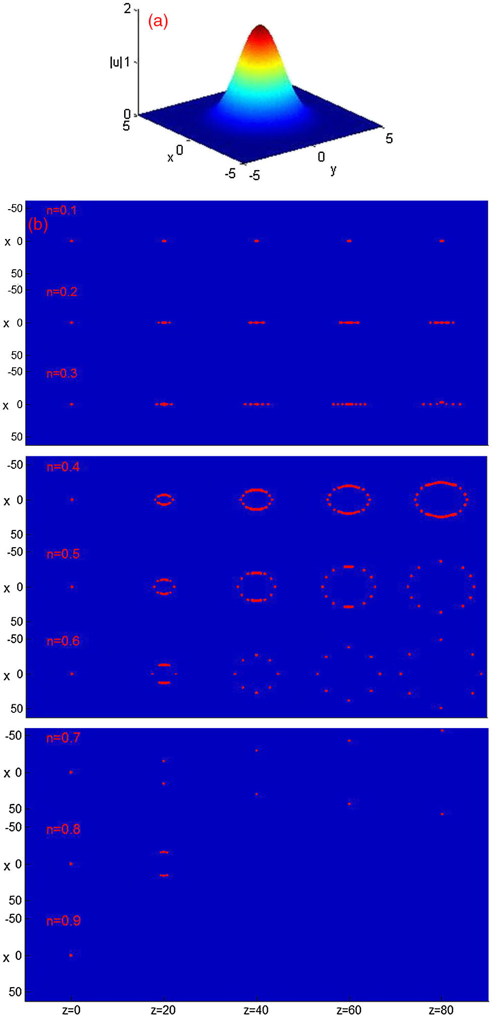
The robustness of the solitons is tested in direct simulations of Eq. (1), with the initial condition multiplied by [ $1 + ρ (x, y)$ ], where $ρ (x, y)$ is a Gaussian random function where $〈 ρ 〉 = 0$ and $〈 ρ^{2} 〉 = σ^{2}$ . The adopted $σ$ is equal to 10% of the soliton amplitude. For this case, the stable soliton solution was obtained using the split-step Fourier method [see Fig. 1(a)]. First, we analyze the propagation dynamics of solitons with various sharpness parameters $n$ for the given parameters, namely, $p = 3$ , $M = 2$ , and $N = 5$ of the EP. For the small and moderate sharpness parameters where $n = 0.1$ , the EP is very weak, and the input soliton is localized on the top of the potential [see Fig. 1(b)]. This is because when the potential is weak, the soliton localization is attributed to the viscous effect that prevents the soliton from falling from the top of potential. This effect obviously differs from that of other well-known models, in which the light beam is easily repulsed at the higher value of the potential well. As the sharpness parameter $n$ of the EP is increased to 0.2 or 0.3, the straight-line arrays can be observed on the second and third lines in Fig. 1(b). Both demonstrate that the EP can provide a continuous source of energy necessary for this, and that the stronger the potential is, the higher the emission rate. As the sharpness of the EP is strong enough, the solitons form a single elliptical ring soliton. During propagation, the elliptical ring soliton gradually expands under the push force of the EP. The expanding velocity of the elliptical soliton ring depends on the sharpness, depth, and ratio of the long axis over the short axis of the potential. As the sharpness and depth of the EP increase, the push force becomes larger, and the elliptical soliton ring expands faster and forms the elliptical soliton arrays. The potential is further increased, and then the solitons decay and lose a large amount of energy. As a result of our extensive numerical simulations, the regions of different soliton dynamics can be obtained by varying $n$ and $p$ , as shown in Fig. 2. The soliton dynamics include soliton localization, soliton straight-line arrays, solitons evolving into either one elliptical ring soliton array or a set of elliptical ring solitons, and soliton decay.

Sign up for Chinese Optics Letters TOC. Get the latest issue of Chinese Optics Letters delivered right to you！Sign up now

Figure 1.(a) Stable soliton solution in Eq. (1). (b) Soliton dynamics for various sharpnesses (from top to bottom: $n = 0.1$ , 0.2, 0.3, 0.4, 0.5, 0.6, 0.7, 0.8, and 0.9) of the elliptical shaped potential when $p = 3$ for $M = 2$ and $N = 5$ . The transverse domain is $(- 50, 50) \times (- 50, 50)$ .

Figure 2.Regions of different soliton dynamics in the plane ( $n$ , $p$ ) when $M = 2$ and $N = 5$ . In region A, for soliton localization; in region B, for soliton straight-line arrays; in regions C and D, for soliton evolution into one elliptical ring soliton array and a set of elliptical ring solitons, respectively; in region E, for soliton decay.

Notice that in the present work, the elliptical shaped potential gives rise to new and dynamic effects for the variety of long and short semi-axes. Figure 3 shows the propagation dynamics of solitons with various long and short semi-axis parameters for the given sharpness parameters, namely, $n = 0.5$ , 0.6, and 0.7 from the top and bottom in every figure. In Fig. 3(a), the elliptical soliton ring gradually expands during propagation, and the solitons are emitted and form soliton arrays for $n = 0.5$ , $M = 3$ , and $N = 5$ . By increasing the sharpness parameter $n$ , a single soliton is completely excited from the elliptical soliton ring under the push force of the EP. For the same sharpness, the solitons form easily when $N = 6$ . However, some solitons decay as the transmission distance increases, as shown in Fig. 3(b). When the long axis is increased to $N = 7$ or $N = 8$ , the propagation dynamics of the solitons are similar to those in Fig. 3(a), but the number of solitons is greater when $N = 7$ and $n = 0.6$ . According to above results, one can see that for the given sharpness and depth of the EP, the ellipse has an optimal ratio of a long elliptical axis over the short axis, which is helpful for the formation of solitons and soliton arrays. For the given sharpness and depth of the EP, the soliton spreads out into an elliptical soliton ring and forms into a single soliton in the gray region. However, it cannot split into a single soliton and soliton arrays in the white region, as is shown in Fig. 4.

Figure 3.Soliton dynamics for various sharpnesses (top: $n = 0.5$ , middle: $n = 0.6$ , bottom: $n = 0.7$ ) of the elliptical shaped potential when $p = 3$ for $M = 3$ and (a) $N = 5$ ; (b) $N = 6$ ; (c) $N = 7$ ; (d) $N = 8$ . The transverse domain is $(- 60, 60) \times (- 60, 60)$ .

Figure 4.Regions of dynamic regimes in the plane ( $M$ , $N$ ) when $p = 3$ and $n = 0.6$ .

Obviously, not only the slope and the depth parameters of the EP but also the parameters of the solitons significantly affect the soliton dynamics. Figure 5 displays the dynamic properties of the solitons arrays for the solitons’ width $(w_{x, y} = 8)$ and given sharpness parameters, namely, $n = 0.5$ , 0.6, and 0.7 from top to bottom in every figure. The solitons can be emitted from a cluster of elliptical ring-shaped patterns even if the EP is weak [see Fig. 5(a)]. As the sharpness of the EP grows stronger and sharper, the soliton is divided into a cluster of elliptical ring solitons [see Fig. 5(b)]. The interesting dynamics demonstrate that the stronger the sharpness parameter $n$ of the EP, the more the elliptical ring expands. In addition, the generation rate of the solitons increases as the value of $n$ increases. When the depth of the EP is too deep, the solitons are split into soliton arrays, but some solitons decay and lose too much energy during propagation [see Fig. 5(c)].

Figure 5.Soliton dynamics for various sharpnesses $n$ = (a) 0.5, (b) 0.6, and (c) 0.7 of the tapered-elliptical potential when $p = 1$ for $M = 2$ and $N = 5$ . The transverse domain is $(- 60, 60) \times (- 60, 60)$ .

In conclusion, we investigate the dissipative spatial solitons in the CQ complex CGL model with elliptical-shaped potentials. The presence of the EP gives rise to some interesting dynamics, including straight-line arrays, the emission of either one elliptical shaped soliton array or several elliptical ring soliton arrays, and soliton decay. In the case of the EP, if the sharpness and depth of the EP are enough strong, the soliton gradually evolves into either one elliptical ring soliton array or a set of elliptical ring solitons with soliton decay. If the sharpness and depth of the EP are moderate, the soliton presents itself in straight-line arrays. If the potential is weak, the solitons cluster on top of the EP. In addition, when the soliton width becomes wider, a cluster of elliptical ring solitons can be obtained for different sharpnesses of the EP. Our results suggest some potential applications, such as routing light signals, all-optical data-processing schemes in optical communication devices, and dynamic and stationary ring-like beams in nonlinear dissipative media.

References

[1] I. S. Aranson, L. Kramer. Rev. Mod. Phys., 74, 99(2002).

[2] L. Ge, M. Shen, T. Zang, L. Dai. Chin. Opt. Lett., 12, 121901(2014).

[3] B. A. Malomed. Nonlinear Schrödinger equations. Encyclopedia of Nonlinear Science(2005).

[4] N. N. Rosanov. Spatial Hysteresis and Optical Patterns(2002).

[5] H. Li. Chin. Opt. Lett., 11, S21902(2013).

[6] H. Li. Chin. Opt. Lett., 12, S11904(2014).

[7] P. Mandel, M. Tlidi. J. Opt. B: Quantum. Semiclass. Opt., 6, R60(2004).

[8] N. Akhmediev, A. Ankiewicz. Dissipative solitons. Lecture Notes in Physics(2005).

[9] D. Mihalache, D. Mazilu, F. Lederer, H. Leblond, B. A. Malomed. Phys. Rev. A., 76, 045803(2007).

[10] D. Mihalache, D. Mazilu, F. Lederer, Y. V. Kartashov, L. C. Crasovan, L. Torner, B. A. Malomed. Phys. Rev. Lett., 97, 073904(2006).

[11] N. N. Rosanov, S. V. Fedorov, A. N. Shatsev. Lecture Notes Phys., 751, 93(2008).