Low-latency deep-reinforcement learning algorithm for ultrafast fiber lasers

Qiuquan Yan; Qinghui Deng; Jun Zhang; Ying Zhu; Ke Yin; Teng Li; Dan Wu; Tian Jiang

doi:10.1364/PRJ.428117

Abstract

The application of machine learning to the field of ultrafast photonics is becoming more and more extensive. In this paper, for the automatic mode-locked operation in a saturable absorber-based ultrafast fiber laser (UFL), a deep-reinforcement learning algorithm with low latency is proposed and implemented. The algorithm contains two actor neural networks providing strategies to modify the intracavity lasing polarization state and two critic neural networks evaluating the effect of the actor networks. With this algorithm, a stable fundamental mode-locked (FML) state of the UFL is demonstrated. To guarantee its effectiveness and robustness, two experiments are put forward. As for effectiveness, one experiment verifies the performance of the trained network model by applying it to recover the mode-locked state with environmental vibrations, which mimics the condition that the UFL loses the mode-locked state quickly. As for robustness, the other experiment, at first, builds a database with UFL at different temperatures. It then trains the model and tests its performance. The results show that the average mode-locked recovery time of the trained network model is 1.948 s. As far as we know, it is 62.8% of the fastest average mode-locked recovery time in the existing work. At different temperatures, the trained network model can also recover the mode-locked state of the UFL in a short time. Remote algorithm training and automatic mode-locked control are proved in this work, laying the foundation for long-distance maintenance and centralized control of UFLs.

1. INTRODUCTION

Artificial intelligence (AI) algorithms studied in the computer field have played a huge role in many other fields [1,2], such as medicine, finance, and optics [3 –5]. The applications of AI mainly include feedback control, pattern recognition, big data analysis, feature extraction, and noise reduction [6 –8]. As an important branch in the field of AI, deep-reinforcement learning (DRL) provides a solution to the feedback-control problem of complex systems because of its perception and decision-making capabilities [9]. Because of this, it is widely used in feedback control in areas such as autonomous driving and industrial automation. When the DRL is applied in different environments, the strategies are different. Therefore, a large number of algorithms based on reinforcement learning have emerged, such as Markov decision process, dynamic programming, Monte Carlo method [10], temporal difference, SARSA, deep $Q$ network (DQN) [11], deep deterministic policy gradient (DDPG) [12], and other algorithms [13]. These algorithms could make the system reach and maintain the desired regime in different environments as soon as possible.

In optics, DRL can also play an important role. Some optical research relies on the stability of the experimental platform or system. Its stability is achieved by adjusting the parameters appropriately according to the current environment. DRL can indirectly collect environmental information and adjust the parameters of the experimental system so that the system quickly reaches and stays in the desired regime for a long time. In this way, the system can work stably without manual adjustment for further research and testing.

In the field of ultrafast photonics, AI has also promoted its development [14,15]. Recently, the combination of machine learning algorithms with the control and characterization of ultrafast dynamics, laser design, and optimization has broken through many technical barriers. Ultrafast fiber laser (UFL) is a significant part of ultrafast photonics research. It can generate femtosecond or picosecond pulses and has been widely used in various applications [16 –23], such as nonlinear optics, precision measurement, and astronomy. The prerequisite for the applications of UFL is to maintain a stable mode-locked state for a long time and to recover quickly once the mode-locked state is disturbed. Fiber lasers based on polarization-maintaining fibers have high stability and do not require polarization controllers to manipulate. Therefore, the UFL in this article refers to the fiber lasers that need to adjust the polarization state to achieve a mode-locked state. To recover the mode-locked state of a UFL, relying solely on manual adjustment of the polarization state is inefficient. Hence, its application is limited. This problem can be solved by automating and accelerating the mode-locked state recovery of the UFL. To realize the automatic control of the polarization state, the electrical polarization controller (EPC) provides technical support [24 –27]. When an EPC is added to the UFL, the voltage values of the multiple EPC channels can be repeatedly adjusted to change the polarization state in the laser cavity and by checking the output of the UFL to obtain the target regime. This is a typical feedback-control process.

Sign up for Photonics Research TOC. Get the latest issue of Photonics Research delivered right to you！Sign up now

Many achievements have been made in the research of automatic mode-locked algorithms for UFL [14,28 –33]. In 2012, Shen et al. [34] applied the pulse counting method to determine the mode-locked state, thereby adjusting the input voltage of the EPC to meet the mode-locked condition. Brunton et al. [35] proposed the concept of self-tuning laser in 2014 and for the first time introduced machine learning algorithms into the automatic mode-locked control of nonlinear polarization rotation (NPR) fiber laser. In the past few years, the Kutz team has demonstrated a number of machine learning algorithms applied to automatic mode-locked control, such as a toroidal search algorithm [36] and recurrent neural network algorithm [37] for mode-locked fiber laser, and a DQN algorithm [38] for NPR fiber laser. Woodward and Kelleher [39] applied a genetic algorithm (GA) to the automatic mode-locked control of the figure-eight laser in 2016. In the second year, they applied GA to the ring fiber laser [40], which was able to obtain a stable and tunable $Q$ switching state. In 2020, Pu et al. [41] proposed a human-like algorithm (HLA) for automatic mode-locked control of NPR fiber laser, which can realize multiple regimes of regulation. They further deployed the algorithm in a field-programmable gate array (FPGA), which greatly improved the response speed of the algorithm to the laser.

Some of the aforementioned automatic mode-locked control algorithms have been verified to be feasible in a simulated environment. However, the verification has not been completed in the actual environment. In addition to the HLA algorithm, other algorithms need to consume at least 30 s or more to reach the target state when they are applied to the actual automatic mode-locked control. Such low-recovery efficiencies are hard to tolerate for practical applications. The HLA algorithm also has a certain defect—when adjusting the polarization state, it only modifies the input voltage of the EPC according to a fixed step. When the randomly initialized polarization state is far away from the target polarization state, the number of adjustment steps could be larger. This leads to an increased time from starting the automatic mode-locked recovery algorithm to resuming the mode-locked state, defined as the recovery time. The average recovery time refers to the average value of the mode-locked recovery time obtained from multiple experiments. According to Ref. [41], the average recovery time with the randomly initializing polarization state method can be about 14 times the fastest recovery time in the HLA algorithm.

A deep-reinforcement learning algorithm with low latency (DELAY) based on the DDPG strategy is introduced for the automatic mode-locked state recovery of the UFLs. The DELAY algorithm mainly includes two actor deep neural networks and two critic deep neural networks. The role of the actor network is to select the appropriate action (corresponding to the input voltages of the EPC) according to the state. The purpose of the critic network is to evaluate the effect of the executed actions on the system. The DELAY algorithm is combined with a UFL based on a saturable absorber (SA) to form an automatic mode-locked control system. In the process of interaction between the algorithm and the environment, a necessary time delay is experienced to ensure that the environment state is stable. The reason is that it takes a certain period of time before the state of the UFL becomes stable after updating the polarization state of the EPC. In experiments, it is found that the fastest fundamental mode-locked (FML) recovery time of the algorithm after vibration is 0.472 s, and the average recovery time is 1.948 s. Compared with the polarization-control algorithms proposed in the past, this algorithm can achieve a large-scale polarization state adjustment in one step, thereby optimizing the solution that the initial polarization state is far from the ideal polarization state. This is the main reason why the DELAY algorithm is faster than the HLA algorithm on average mode-locked recovery time. In addition, the data between the computer and the EPC-controlled unit/the laser output monitoring device in this system are transmitted through a wireless network. The DELAY algorithm is deployed on the computer, so this means that the system can realize remote automatic mode-locked control. The realization of remote control indicates that the system can realize remote maintenance and monitoring. It is also convenient for remote assistance to adjust the system status. Finally, a computer can control multiple laser systems simultaneously, which is of great significance to the debugging and controlling of the cascade system.

The organization of the paper is as follows. A low-latency deep-reinforcement learning algorithm is presented for automatic mode-locked state recovery for UFL in Section 2. Then, in Section 3, the architecture of the UFL and a feedback-control system are introduced. Related characterization of the system is also mentioned. In Section 4, the experimental results of the deployment of the algorithm in the system are demonstrated, which mainly include the vibration test and temperature test. In Section 5, the contributions and prospects are discussed.

2. LOW-LATENCY DEEP-REINFORCEMENT LEARNING ALGORITHM

The structure of the DELAY algorithm is illustrated in Fig. 1. It depicts four deep neural networks, including two actor networks (in black) with the same structure and two critic networks (in red) with the same structure. The actor networks are constructed by a three-layer fully connected deep neural network, in which the number of nodes in the two hidden layers is 256, and the input layer and output layer are state and action, respectively. The function in the algorithm is to infer the next action based on the current state to ensure that the system reaches the target regime as soon as possible. The above actor network interacts with the laser environment directly and determines the voltage values given to the EPC in the next step according to the current laser state. The following target actor network can be considered as a replicated version of the actor network, which is used to calculate and estimate possible future actions. The critic networks are also constructed by a three-layer fully connected deep neural network, in which the number of nodes in the two hidden layers is set to 256. The input layer is the state and the action to be performed, and the output layer is a $Q$ value for evaluating the reward of the action in the laser environment. The above critic network is used to calculate the $Q$ value of the currently executed action. The following target critic network is used to compute the $Q$ value corresponding to the action obtained from the target actor network.

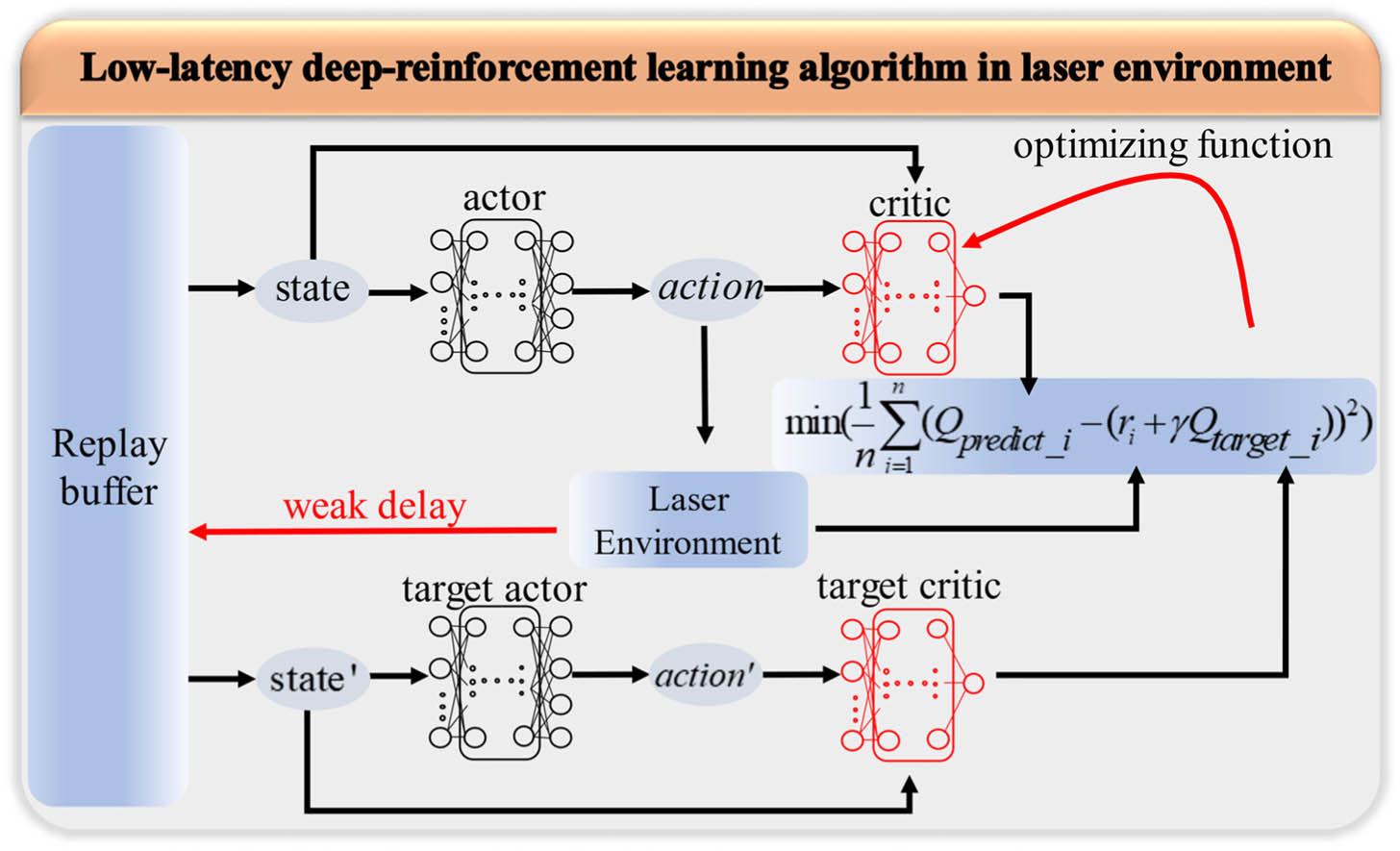
Structure of the low-latency deep-reinforcement learning algorithm based on DDPG strategy in the laser environment.

Figure 1.Structure of the low-latency deep-reinforcement learning algorithm based on DDPG strategy in the laser environment.

The replay buffer in Fig. 1 stores a large number of tuples ( $s$ , $a$ , $r$ , $s^{'}$ , done), where $s$ represents the current state, $a$ is the action selected by the actor network according to $s$ , $r$ means the reward for performing the action $a$ , $s^{'}$ indicates the state after executing $a$ , and done indicates whether the target regime is reached after executing $a$ . It is used as a training set for network training in the algorithm. Since the network training process randomly selects samples from the replay buffer, the correlation between adjacent actions is broken up. In this way, the training effect of the network can be improved. The purpose of the weak delay in Fig. 1 is that when the action is executed, it needs to be read after the state of the laser is stable for 0.5 s. In this way, the polarization state of the laser can be judged more accurately.

The algorithm is mainly used to train a deep neural network model so that the polarization state can be quickly adjusted after the mode-locked state being disturbed. For DRL algorithms, the quality of the environment definition has a great impact on the performance of the algorithm, so the abstraction of states and actions in the environment needs to be carefully considered. In the DELAY algorithm, the state is defined as a six-tuple, including the four-channel voltage values of the EPC in the current state, two pulse-stability evaluation values obtained according to the laser output signals in the time domain and frequency domain. The calculation method of those two values will be given in Section 3. The action is defined as a four-tuple, corresponding to the four-channel input voltage values of the EPC. To make the training model more effective, the voltage values applied to the EPC are mapped to [ $- 1$ , 1]. Since the accuracy of the EPC voltage setting is 0.001, the approximate value of the algorithm result can be used when setting the voltage value for the EPC.

In the DELAY algorithm, the actor and critic networks need to be trained through a backpropagation method. The loss function of the actor network is defined as ${loss}_{a} = \frac{1}{n} \sum_{j = 1}^{n} Q_{predict_j} = \frac{1}{n} \sum_{j = 1}^{n} critic (s_{j}, a_{j}),$ (1)where $n$ means the number of tuples in the replay buffer used when calculating a loss value, and $s_{j}$ and $a_{j}$ are from the replay buffer. The loss function of the critic network is ${loss}_{c} = \frac{1}{n} \sum_{i = 1}^{n} {[Q_{predict_i} - (r_{i} + γ Q_{target_i})]}^{2},$ (2)where $n$ has the same meaning as $n$ in Eq. (1), $r_{i}$ means the reward obtained from the recorded execution of the $i$ th action, $Q_{predict_i}$ represents the result obtained from the critic network, the discount factor $γ$ is the weight of the next action value, and $Q_{target_i}$ indicates the prediction result obtained in the target critic network. The parameter update method of the target actor and the target critic network is as follows: ${\begin{matrix} ω_{a_t}^{'} = τ ω_{a_t} + (1 - τ) ω_{a_new} \\ θ_{c_t}^{'} = τ θ_{c_t} + (1 - τ) θ_{c_new} \end{matrix},$ (3)where $ω_{a_t}$ and $ω_{a_t}^{'}$ , respectively, indicate the weight parameters before and after the target actor network is updated, and $ω_{a_new}$ means the updated weight parameters of the actor network. The second formula corresponds to the parameters in the critic network and the target critic network. This method of parameter update is called soft update, which helps the model convergence process to be more stable. $τ$ represents the soft-update weight.

In the training process of the network model, the hyperparameter settings in the networks are shown in Table 1. The $actor_l r$ and $critic_l r$ are the learning rate of the actor network and the critic network, respectively. The $buf fer_size$ is the size of the replay buffer, and the $batch_size$ is the training batch size. The training and optimizing processes of the algorithm model are completed in combination with the actual UFL system. At the beginning of each iteration, the four input voltages of the EPC are randomly initialized. Then, the actor network is used to calculate the next action ( $a$ ) based on the current state ( $s$ ), and the EPC input voltages are updated. After 0.5 s, the new state ( $s^{'}$ ) and the reward ( $r$ ) of the system are obtained from the laser environment, and the tuple ( $s$ , $a$ , $r$ , $s^{'}$ , done) is stored in the replay buffer. When the system reaches the target FML state, an iteration process is considered to be over. In a model training process, this iterative process needs to be repeated 100 times. In the iterative process, the weight parameters of the actor and critic networks are periodically trained and updated. The other two target networks have also been soft updated accordingly. The goal of parameters update is to minimize the number of steps from the initial state to the mode-locked state in an iteration process. When the network model still cannot reach the target regime quickly after the iteration, the network is trained again on the basis of the current trained model.Table 1.

Hyperparameters in the Training Process

Hyperparameter	Value	Hyperparameter	Value
$actor_l r$	$10^{- 6}$	$critic_l r$	$10^{- 6}$
$γ$	0.99	$τ$	0.02
$buf fer_size$	100	$batch_size$	8

Figure 2 shows the flow chart using the trained actor network model to maintain the stable mode-locked state of the UFL. The stabilization algorithm reads the time–frequency-domain information output by the laser from the oscilloscope. After that, a certain strategy (introduced in Section 3) is used on the computer to determine whether the laser has reached the mode-locked state. If the system is in the mode-locked state, wait for 0.5 s before the computer reads the oscilloscope data again. Otherwise, the computer runs the trained actor network model to calculate the action to be performed. Then, the action is converted into four voltage values and assigned to the four voltage input ports of the EPC. After waiting for 0.1 s, the system enters a new round of the iterative process. The program can run all of the time to monitor and maintain the stable mode-locked state of the system.

Figure 2.Flow chart for stable mode-locked state monitoring.

Table 2 shows the comparison of different algorithms in mode-locking time applied to the fiber laser, where EA represents the evolutional algorithm and PSO means the particle swarm optimization algorithm. The last three sets of results are all tested in the system built by this work. From the results in the table, the DELAY algorithm has the best performance in average recovery time. However, as of the current experimental results, the fastest mode-locked recovery time of the DELAY algorithm can only reach 0.472 s, which is 0.252 s slower than the HLA algorithm, which is because the process of transmitting four voltage values from the computer to the FPGA is completed through the wireless network. According to thousands of statistics, the average time it takes to update the input voltages of the EPC is about 0.524 s each time. Therefore, the time cost of the DELAY algorithm is relatively longer. But for practical applications, adjusting the laser to the mode-locked state within 2 s on average can meet real-time requirements.Table 2.

Comparison of Different Algorithms in Mode-Locking Time

Algorithm Name		Time
GA [39]		$\sim 30 \min$ mode-locking time
EA [42]		$\sim 30 \min$ mode-locking time
GA [24]		$\sim 30 s$ recovery time
HLA [41]		0.22 s fastest recovery time 3.1 s average recovery time
Running on this system	GA	377 s average recovery time
	PSO	216 s average recovery time
	DELAY	0.472 s fastest recovery time 1.948 s average recovery time

All of the implemented algorithms are written in Python language and run on a laptop with Windows 10 operating system. The model of the CPU is Intel Core i5-8265U @ 1.6 GHz in the laptop. The DELAY algorithm is implemented based on the PyTorch 1.7 framework [43].

3. EXPERIMENTAL SETUP

To demonstrate the effectiveness and the robustness of the DELAY algorithm, a UFL is constructed, as shown in Fig. 3. The UFL consists of a wavelength-division multiplexer (WDM) that reflects the 980 nm light, a piece of 0.4 m erbium-doped fiber (EDF) that serves as gain medium pumped by a 980 nm laser diode, an EPC used to adjust the intracavity polarization, a fiber SA based on single-walled carbon nanotube SA (SWCNT) film [44,45], and a 10/90 optical coupler (OC). The 90% port of the optical power is fed back into the cavity, while the 10% port is used for the output. The total length of the cavity is $\sim 5.24 m$ .

Figure 3.Experimental setup of UFL based on SA. WDM, 980/1550 nm wavelength division multiplexer; EDF, erbium-doped fiber; EPC, electrical polarization controller; FPGA, field-programmable gate array; SA, saturable absorber; OC, optical coupler; ISO, isolator; PD, photodetector.

There are four channels on the EPC for voltage adjustment to change the polarization state. The voltage adjustment range of each channel is 0–5 V, and the corresponding angle adjustment range is 0–4π rad. The four channels of the EPC in the system are connected to the 4 digital–analog converter (DAC) output ports of the FPGA. Corresponding to the FPGA, the minimum amplitude of angle adjustment on each channel is $π / 625, 000 rad$ . When the input voltages of the EPC need to be adjusted, a computer can send the voltage data stream to the FPGA. After the FPGA receives the data stream, it can immediately update the voltage values of the four EPC channels. In this way, the polarization state of the system can be controlled by the computer. By using a polarization-measuring instrument to record the polarization state, proper adjustment of the input voltage of the EPC can traverse the entire surface of the Poincaré sphere. It is a feature of the EPC that the arbitrary change of the adjustment step in the DELAY algorithm can be realized. Therefore, no matter how far the position of the output polarization state in the fiber laser deviates from the polarization state of the mode-locked state, it can be returned to the target state with a few adjustment steps. This is one of the important reasons why the average mode-locked recovery time obtained by the DELAY algorithm is much lower than that of other algorithms.

In the research, first, by manually adjusting the polarization range of the EPC, the UFL can work in the FML state. As illustrated in Fig. 4, when the system is under the FML state, the pulse period is 25.34 ns in laboratory time, and the repetition frequency ( $f_{rep}$ ) is 39.46 MHz. Figure 4(c) shows the autocorrelation information of the mode-locked pulse. Through ${sech}^{2}$ function fitting, the pulse width is found to be about 316 fs. Figure 4(d) plots the output spectrum, which indicates a center wavelength of 1560.77 nm. The ${sech}^{2}$ -like spectrum illustrates that the UFL behaves in a typical soliton mode-locked state. The results presented are all measured at room temperature (about 25°C).

Figure 4.Characterization of the output when the laser is in the FML state. (a) Time-domain pulse output within 0.2 μs laboratory time. The pulse interval is 25.34 ns. (b) Frequency-domain signal characterization in 4 GHz bandwidth. The $f_{rep}$ is 39.459 MHz. (c) The pulse autocorrelation and the result of fitting using ${sech}^{2}$ function. (d) The spectrum of the laser output.

Subsequently, the computer is connected with the oscilloscope and the FPGA through a wireless network. In this way, the computer can collect the output of the laser to provide feedback for the DELAY algorithm and change the polarization state of the EPC by transmitting new voltage values to the FPGA. Specifically, the oscilloscope transmits the collected time-domain signal and the processed frequency-domain signal to the computer so that the algorithm can determine whether the UFL reaches the mode-locked state. After the DELAY algorithm processes the data in the current state, a new set of voltage values will be transmitted from the computer to the FPGA to update the polarization state of the EPC. The output arm of the UFL is first connected with an InGaAs photodetector (PD) with a bandwidth greater than 10 GHz to detect the pulse signal. Then, the pulse signal is monitored and recorded by the oscilloscope with a bandwidth of 4 GHz. The oscilloscope and the FPGA that controls the EPC are connected to the router through their own network ports. The computer wirelessly communicates with the oscilloscope and the FPGA through the form of the wireless network. In this system, it is simple to remotely realize the monitoring of the system status and the automatic mode-locked control.

The computer sends read instructions to the oscilloscope to read fixed-length time–frequency-domain data. The reading length of the time-domain signal is 4 μs, and the reading range of the frequency-domain signal is set to 0–3.75 GHz. After receiving the read instructions, the oscilloscope transmits the currently collected time-domain data and processed frequency-domain data to the computer. Next, the computer executes the corresponding mode discrimination program to determine whether the system is in the FML state. In this work, there are three formulas in the program to determine the status of the system. The first equation characterizes the stability of the time-domain signal, and its form is ${cost}_{time} = {\begin{matrix} 20 & if n (t_p) \neq n_{t_lock} \\ std (t_p) + abs (avg_t_p_{cur} - avg_t_p_{lock}) & else \end{matrix},$ (4)where $t_p$ represents the peak sequence of time-domain pulse data within 4 μs, $n$ is the length of $t_p$ , $n_{t_lock}$ means the number of pulses within 4 μs laboratory time, std denotes the operator for taking variance, abs is the absolute value operation, and $avg_t_p_{cur}$ and $avg_t_p_{lock}$ , respectively, mean the average values of the time-domain peak sequence in the current state and the FML state. The $t_p$ is obtained by processing the time-domain pulse sequence collected from the oscilloscope using the peak-finding algorithm, which shows the intensity and quantity of the time-domain pulse output from the fiber laser in the current state. The lowest threshold of the peak-finding algorithm needs to be selected appropriately to ensure that the peak point of the mode-locked pulse could be searched. When the ${cost}_{time}$ is smaller, the output pulse is more stable.

The second equation reflects the stability of the frequency comb, and its expression is ${cost}_{freq} = {\begin{matrix} 20 & if n (f_p) \neq n_{f_lock} \\ std (f_p) + abs (min_f_p_{cur} / avg_f_p_{lock}) & else \end{matrix},$ (5)where the variables and functions are similar to those expressed in Eq. (4), except that the parameters correspond to the frequency domain. The $f_p$ is the peak sequence of frequency-domain pulse data in the range of 0–3.75 GHz, which is calculated by the oscilloscope. By comparing $f_p$ with the peak sequence of frequency-domain data under the stable mode-locked state, its mean and variance will reflect the mode-locking stability of the fiber laser in the current state. $n_{f_lock}$ represents the number of comb teeth of the mode-locked pulsed optical frequency comb in the range of 0–3.75 GHz. Similarly, when the value of ${cost}_{freq}$ is smaller, the frequency comb is more uniform and steadier.

The last function combines time–frequency information to give a quantitative FML state judgment standard; the expression is as follows: $r = 20 - ({cost}_{time} + {cost}_{freq}),$ (6)where the system is considered to be in the stable FML state when the $r$ reaches 5 or more. Otherwise, the system is considered to be not in the FML state. This quantitative judgement comes from a large number of experimental tests and empirical analysis. The value is also used in the action reward. In the DELAY algorithm, the reward is defined as the sum of $r$ obtained by adjusting the polarization state multiple times in one iteration. The idea to define reward function mainly comes from two aspects. On the one hand, the definition of $r$ can well reflect the target state to be achieved by the system. This helps the algorithm to quickly distinguish the different states of the system and ensures the effectiveness of the algorithm. On the other hand, the parameters that need to be measured in the reward function are only the time-domain and frequency-domain data of the laser output detected by the PD, which can be shown in real time by an oscilloscope. The use of parameters that can be obtained in real time to define a cost function can improve the efficiency of the algorithm.

Figure 5 sketches the time-domain and frequency-domain signal output by the laser in different polarization states, which are FML and $Q$ switch mode-locked states. The laser pulse signal in the time-frequency domain in the FML state has high flatness, and the number of pulses in a certain time-frequency range is fixed. The time-domain signal in the $Q$ switched mode-locked state is uneven, and the number of pulses is also unstable. In addition, the laser output has many other states, such as second-harmonic mode-locked state, third-harmonic mode-locked state, and $Q$ switching state. In most non-FML states, the numbers of time-domain pulses and frequency-domain combs collected by oscilloscope are not equal to the corresponding values in the FML state. Therefore, the value of $r$ in these states is usually $- 20$ . By comparing the actual state of the oscilloscope with the program processing results, it is found that the corresponding reward value is greater than 5 when the UFL is in the stable FML state. When the system is in other states, the $r$ value will be lower than 5. Within the value range of $r$ , the larger the value, the more stable the FML state of the system. The smaller the value of $r$ , the further the system state deviates from the FML state. Therefore, Eq. (6) is used for the reward definition of the laser environment in the DELAY algorithm.

Figure 5.Comparison of the time-domain and frequency-domain signal output by the laser in different polarization states. From left to right: FML state and $Q$ switch mode-locked state. In each column, the top row shows the time-domain signal within 40 μs laboratory time, and the bottom plot is the frequency-domain signal within the 4 GHz bandwidth.

4. RESULTS AND DISCUSSION

After completing the design and implementation of the algorithm, two tests are carried out. The external factors that affect the mode-locked state of the UFL are mainly environmental vibrations and large changes in temperature. On the one hand, the motor vibration is applied to simulate the environmental vibrations so as to quickly disturb the mode-locked state of the UFL. Then the DELAY algorithm is used to verify whether the mode-locked state can be quickly recovered. On the other hand, the UFL is controlled at different temperatures to test whether the DELAY algorithm can train a suitable model for automatic mode-locked state recovery. This will provide a solution to realize the automatic mode-locked state recovery when the temperature change causes the UFL to lose the mode-locked state slowly. The experimental results are given from the two parts separately.

A. Vibration Test

Generally, sudden vibration has a great influence on the polarization state of the UFL. When severe jitter is applied to the laser, the FML state is generally easily lost. Even if the jitter is stopped, it is difficult for the laser to recover the FML state automatically. To verify the effect of the algorithm in recovering the mode-locked state when the sudden jitter causes the mode-locked state to disappear, a large number of experiments are carried out.

To expand the range of the laser jitter, all of the cavity parts of the laser except EPC and its pigtails are put in a $14 cm \times 13.5 cm \times 5 cm$ aluminum box. A motor with a voltage of 5 V and a limited current of 0.12 A is attached to the surface of the aluminum box to introduce vibrations. By verification, it is found that when the vibration time reaches 1.5 s, the FML state of the laser cannot be automatically recovered. A relay is used to power the motor so that the experiment could be executed many times without manual operation. The program written in Python language is used to realize the control of the motor power switch by sending instructions. Therefore, both the time and the interval of motor vibrations can be controlled by the program without manual intervention.

Before performing the test experiment of recovering the mode-locked state after vibration, a model of the DELAY algorithm in the experimental environment was trained. Figure 6(a) shows the record of the variation of the reward value of the algorithm model during the last 100 iterations. In the last 30 training sessions, the reward value basically remained near 0. This implies that the trained model can find the mode-locked state quickly. After the entire algorithm models are trained, the actor model is used in the automatic mode-locked state recovery algorithm.

Figure 6.Effect diagram of algorithm recovery after the laser loses mode-locked state due to motor vibration. (a) The convergence curve of the reward value in the last 100 rounds of stable mode-locked calculation model-training iterations. (b) The $f_{rep}$ and power change of the laser output during the process of applying vibration to the laser and starting the recovery algorithm. (c) The recovery time statistics of 1500 vibration tests. (d) The output $f_{rep}$ and power change of the system within 10 min under the condition of vibrating for 1.5 s per minute and running the mode-locked recovery algorithm all of the time.

In addition, the influence of motor vibration on the FML state of the fiber laser is tested. In the experiment, the motor is controlled to vibrate for 1.5 s after the system is in a stable FML state for 120 s. Within 60 s after the motor vibrates, there is no external disturbance to the system. During this process, the output of the system has been recorded by the power meter and frequency meter. As illustrated in Fig. 6(b), within 60 s after vibration, the system has not been in the FML state. At the moment of 180 s, the mode-locked recovery algorithm is started. It is shown in the figure that after the algorithm is started, the system recovers the FML state in a short time. Moreover, the system can maintain a stable output power and $f_{rep}$ since then. This process confirmed that motor vibration can disturb the mode-locked state of the UFL. The process also shows that the DELAY algorithm can recover the FML state of the laser, which reflects the effectiveness of the algorithm.

To test the performance of the algorithm to recover the mode-locked state in the system, more than 1500 experiments were carried out. In each experiment, the operating state of the mode-locked recovery algorithm is maintained, and the system output power and $f_{rep}$ are continuously recorded. The vibration frequency of the motor is set to once per minute. These operations are controlled by the program. Figure 6(c) shows the counts of the number of different mode-locked recovery time intervals. Among them, the number of times of resuming the mode-locked state within 3 s accounted for 88.15% of the total number of experiments. After the system loses mode-locked state due to vibration, the average mode-locked recovery time is 1.948 s, and the fastest recovery time tested in the experiment is 0.472 s.

Figure 6(d) shows the changes in $f_{rep}$ and output power of the system within 10 min during the experimental tests. The motor vibrates continuously for 1.5 s per minute. After the algorithm detects signal fluctuations in the time-frequency domain, it will immediately search for a new polarization state for the UFL to recover the mode-locked state of the system. Every time the system loses the mode-locked state due to motor vibration, it can quickly recover the mode-locked state under the correction of the algorithm. During the period of no vibration interference, the system can maintain a stable mode-locked state. This means that the polarization state found by the mode-locked recovery algorithm could make the system maintain a stable FML state.

B. Temperature Test

It is known that when the experimental temperature changes greatly, the intracavity polarization distributions of the UFL will also be changed slowly. This means that the actor network model trained at room temperature might not adapt to various temperature conditions. A feasible solution is to train appropriate actor network models at different temperatures. According to the temperature in the laser cavity, applying a corresponding trained actor network model can recover the stable mode-locked state quickly. Through experimental verification, the model trained at room temperature (25°C) is not applicable in environments where the temperature exceeds 30°C or is below 20°C. Therefore, a set of experiments are designed to train the algorithm every 5°C in the range of 15°C–40°C.

Figure 7 presents the results of the DELAY algorithm training at different temperatures. According to statistics, the number of network model training iterations at each temperature is mostly 300 or 400. It can be seen that in the last 30 rounds of network model training at each temperature, the reward value of the system tends to stabilize. This shows that these models can already be used for automatic mode-locked state recovery. At different temperatures, the motor is used to disturb the polarization state of the laser to test the effectiveness of the trained model. The results show that all trained models can recover the FML state of the system at the corresponding temperature.

Figure 7.Changes in the reward value of the designed algorithm model in the system at different temperatures. (a)–(f) are the results of the last 100 rounds of training recorded from 15°C to 40°C.

Table 3 shows the statistical results of the average mode-locked state recovery time of the trained model at different temperatures, where 10 times of mode-locked state recovery tests were performed at each temperature. As a result, the statistics at different temperatures are all in about 2 s, and their difference is negligible.Table 3.

Average Mode-Locked State Recovery Time at Different Temperatures

Temperature (°C)	15	20	25
Time (s)	1.616	1.869	2.163
Temperature (°C)	30	35	40
Time (s)	1.951	2.489	1.645

The experiment verifies the robustness of the DELAY algorithm, i.e., the algorithm can adapt to a variety of temperature environments. Combined with the trained network models at different temperatures, automatic mode-locked state recovery can be realized in a real temperature-varied environment. By monitoring the temperature of the environment in real time, a suitable model can be selected to recover the mode-locked state of the UFL. In this way, the DELAY algorithm can be used to automatically recover the mode-locked state even when the ambient temperature changes significantly.

5. CONCLUSIONS

In this paper, a low-latency deep-reinforcement learning algorithm based on the DDPG strategy was proposed and implemented for automatic mode-locked control of UFL. Based on the DELAY algorithm and the UFL, an automatic mode-locked control system was built to maintain and monitor the FML state of the laser. Experimental results show that the DELAY algorithm can recover the FML state of the laser in an average of 1.948 s after the laser loses its mode-locked state due to the motor vibration, which is 62.8% of the fastest average recovery time in the past research to the best of our knowledge. The shortest mode-locked state recovery time in the system is 0.476 s. Meanwhile, the DELAY algorithm realizes fast mode-locked state recovery of the UFL when the system is at any ambient temperature of 15°C–40°C. Equally important, since the data feedback between the DELAY algorithm and the laser in the system is completed through the wireless network, the system can realize remote mode-locked control. This means that this system can be used in unmanned scenarios to complete important functions such as distance measurement and gas detection. Furthermore, the remote-control feature makes the system conducive to the large-scale centralized control of multiple UFLs. The DELAY algorithm is also applicable to other actual systems with feedback delays. The source code of the implemented algorithm has been opened in Gitee [46], which encourages others to use, modify, and add new solutions.

References

[1] T. Zhou, L. Fang, T. Yan, J. Wu, Y. Li, J. Fan, H. Wu, X. Lin, Q. Dai. In situ optical backpropagation training of diffractive optical neural networks. Photon. Res., 8, 940-953(2020).

[2] Y. Chang, H. Wu, C. Zhao, L. Shen, S. Fu, M. Tang. Distributed Brillouin frequency shift extraction via a convolutional neural network. Photon. Res., 8, 690-697(2020).

[3] Z. Tao, J. Zhang, J. You, H. Hao, H. Ouyang, Q. Yan, S. Du, Z. Zhao, Q. Yang, X. Zheng, T. Jiang. Exploiting deep learning network in optical chirality tuning and manipulation of diffractive chiral metamaterials. Nanophotonics, 9, 2945-2956(2020).

[4] B. J. Shastri, A. N. Tait, T. Ferreira de Lima, W. H. P. Pernice, H. Bhaskaran, C. D. Wright, P. R. Prucnal. Photonics for artificial intelligence and neuromorphic computing. Nat. Photonics, 15, 102-114(2021).

[5] H. Lin, J. Xie, T. Fan, Y. He, J. Chen, H. Zhang, S. Zhuo. Rapid prediction of drug inhibition under heat stress: single-photon imaging combined with a convolutional neural network. Nanoscale, 12, 23134-23139(2020).

[6] Z. Tao, J. You, J. Zhang, X. Zheng, H. Liu, T. Jiang. Optical circular dichroism engineering in chiral metamaterials utilizing a deep learning network. Opt. Lett., 45, 1403-1406(2020).

[7] J. Li, D. Mengu, Y. Luo, Y. Rivenson, A. Ozcan, T. Jiang. Class-specific differential detection in diffractive optical neural networks improves inference accuracy. Adv. Photon., 1, 046001(2019).

[8] S. Feng, Q. Chen, G. Gu, T. Tao, L. Zhang, Y. Hu, W. Yin, C. Zuo. Fringe pattern analysis using deep learning. Adv. Photon., 1, 025001(2019).

[9] Y. Li. Deep reinforcement learning: an overview(2017).

[10] J. Ma, Z. Piao, S. Huang, X. Duan, G. Qin, L. Zhou, Y. Xu. Monte Carlo simulation fused with target distribution modeling via deep reinforcement learning for automatic high-efficiency photon distribution estimation. Photon. Res., 9, B45-B56(2021).

[11] V. Mnih, K. Kavukcuoglu, D. Silver, A. A. Rusu, J. Veness, M. G. Bellemare, A. Graves, M. Riedmiller, A. K. Fidjeland, G. Ostrovski, S. Petersen, C. Beattie, A. Sadik, I. Antonoglou, H. King, D. Kumaran, D. Wierstra, S. Legg, D. Hassabis. Human-level control through deep reinforcement learning. Nature, 518, 529-533(2015).

[12] T. P. Lillicrap, J. J. Hunt, A. Pritzel, N. Heess, T. Erez, Y. Tassa, D. Silver, D. Wierstra. Continuous control with deep reinforcement learning(2015).

[13] Y. Han, S. Xiang, Y. Wang, Y. Ma, B. Wang, A. Wen, Y. Hao. Generation of multi-channel chaotic signals with time delay signature concealment and ultrafast photonic decision making based on a globally-coupled semiconductor laser network. Photon. Res., 8, 1792-1799(2020).

[14] G. Genty, L. Salmela, J. M. Dudley, D. Brunner, A. Kokhanovskiy, S. Kobtsev, S. K. Turitsyn. Machine learning and applications in ultrafast photonics. Nat. Photonics, 15, 91-101(2020).

[15] G. Pu, L. Zhang, W. Hu, L. Yi. Automatic mode-locking fiber lasers: progress and perspectives. Sci. China Inf. Sci., 63, 160404(2020).

[16] T. Jiang, K. Yin, C. Wang, J. You, H. Ouyang, R. Miao, C. Zhang, K. Wei, H. Li, H. Chen, R. Zhang, X. Zheng, Z. Xu, X. Cheng, H. Zhang. Ultrafast fiber lasers mode-locked by two-dimensional materials: review and prospect. Photon. Res., 8, 78-90(2020).

[17] K. Yin, Y. Li, Y. Wang, X. Zheng, T. Jiang. Self-starting all-fiber PM Er:laser mode locked by a biased nonlinear amplifying loop mirror. Chin. Phys. B, 28, 124203(2019).

[18] J. Zou, C. Dong, H. Wang, T. Du, Z. Luo. Towards visible-wavelength passively mode-locked lasers in all-fibre format. Light Sci. Appl., 9, 61(2020).

[19] X. Zhao, T. Li, Y. Liu, Q. Li, Z. Zheng. Polarization-multiplexed, dual-comb all-fiber mode-locked laser. Photon. Res., 6, 853-857(2018).

[20] R. Miao, M. Tong, K. Yin, H. Ouyang, Z. Wang, X. Zheng, T. Jiang. Soliton mode-locked fiber laser with high-quality MBE-grown Bi₂Se₃ film. Chin. Opt. Lett., 17, 071403(2019).

[21] W. Li, C. Zhu, X. Rong, J. Wu, H. Xu, F. Wang, Z. Luo, Z. Cai. Bidirectional red-light passively Q-switched all-fiber ring lasers with carbon nanotube saturable absorber. J. Lightwave Technol., 36, 2694-2701(2018).

[22] J. Liu, J. Wu, H. Chen, Y. Chen, Z. Wang, C. Ma, H. Zhang. Short-pulsed Raman fiber laser and its dynamics. Sci. China Phys. Mech. Astron., 64, 214201(2020).

[23] D. Huang, C. Shang, F. Li, Z. Cheng, X. Zhang, Z. Kang, X. Feng, P. Wai. Discrete Fourier domain harmonically mode locked laser by mode hopping modulation. 24th Opto-Electronics and Communications Conference (OECC) and International Conference on Photonics in Switching and Computing (PSC), 1-3(2019).

[24] D. G. Winters, M. S. Kirchner, S. J. Backus, H. C. Kapteyn. Electronic initiation and optimization of nonlinear polarization evolution mode-locking in a fiber laser. Opt. Express, 25, 33216-33225(2017).

[25] G. Pu, L. Yi, L. Zhang, W. Hu. Genetic algorithm-based fast real-time automatic mode-locked fiber laser. IEEE Photon. Technol. Lett., 32, 7-10(2019).

[26] G. Pu, L. Yi, L. Zhang, C. Luo, Z. Li, W. Hu. Intelligent control of mode-locked femtosecond pulses by time-stretch-assisted real-time spectral analysis. Light Sci. Appl., 9, 13(2020).

[27] U. Andral, J. Buguet, R. S. Fodil, F. Amrani, F. Billard, E. Hertz, P. Grelu. Toward an autosetting mode-locked fiber laser cavity. J. Opt. Soc. Am. B, 33, 825-833(2016).

[28] X. Fu, J. N. Kutz. High-energy mode-locked fiber lasers using multiple transmission filters and a genetic algorithm. Opt. Express, 21, 6526-6537(2013).

[29] A. Kokhanovskiy, A. Bednyakova, E. Kuprikov, A. Ivanenko, M. Dyatlov, D. Lotkov, S. Kobtsev, S. Turitsyn. Machine learning-based pulse characterization in figure-eight mode-locked lasers. Opt. Lett., 44, 3410-3413(2019).

[30] T. Hellwig, T. Walbaum, P. Groß, C. Fallnich. Automated characterization and alignment of passively mode-locked fiber lasers based on nonlinear polarization rotation. Appl. Phys. B, 101, 565-570(2010).

[31] S. L. Brunton, X. Fu, J. N. Kutz. Extremum-seeking control of a mode-locked laser. IEEE J. Quantum Electron., 49, 852-861(2013).

[32] J. N. Kutz, S. L. Brunton. Intelligent systems for stabilizing mode-locked lasers and frequency combs: machine learning and equation-free control paradigms for self-tuning optics. Nanophotonics, 4, 459-471(2015).

[33] F. Meng, J. M. Dudley. Toward a self-driving ultrafast fiber laser. Light Sci. Appl., 9, 26(2020).

[34] X. Shen, W. Li, M. Yan, H. Zeng. Electronic control of nonlinear-polarization-rotation mode locking in Yb-doped fiber lasers. Opt. Lett., 37, 3426-3428(2012).

[35] S. L. Brunton, X. Fu, J. N. Kutz. Self-tuning fiber lasers. IEEE J. Sel. Top. Quantum Electron., 20, 464-471(2014).

[36] X. Fu, S. L. Brunton, J. N. Kutz. Classification of birefringence in mode-locked fiber lasers using machine learning and sparse representation. Opt. Express, 22, 8585-8597(2014).

[37] T. Baumeister, S. L. Brunton, J. N. Kutz. Deep learning and model predictive control for self-tuning mode-locked lasers. J. Opt. Soc. Am. B, 35, 617-626(2018).

[38] C. Sun, E. Kaiser, S. L. Brunton, J. N. Kutz. Deep reinforcement learning for optical systems: a case study of mode-locked lasers. Mach. Learn. Sci. Technol., 1, 045013(2020).

[39] R. Woodward, E. J. Kelleher. Towards ‘smart lasers’: self-optimisation of an ultrafast pulse source using a genetic algorithm. Sci. Rep., 6, 37616(2016).

[40] R. I. Woodward, E. J. R. Kelleher. Genetic algorithm-based control of birefringent filtering for self-tuning, self-pulsing fiber lasers. Opt. Lett., 42, 2952-2955(2017).

[41] G. Pu, L. Yi, L. Zhang, W. Hu. Intelligent programmable mode-locked fiber laser with a human-like algorithm. Optica, 6, 362-369(2019).

[42] U. Andral, R. S. Fodil, F. Amrani, F. Billard, E. Hertz, P. Grelu. Fiber laser mode locked through an evolutionary algorithm. Optica, 2, 275-278(2015).

[43] A. Paszke, S. Gross, F. Massa, A. Lerer, J. Bradbury, G. Chanan, T. Killeen, Z. Lin, N. Gimelshein, L. Antiga. PyTorch: an imperative style, high-performance deep learning library(2019).

[44] A. Martinez, Z. Sun. Nanotube and graphene saturable absorbers for fibre lasers. Nat. Photonics, 7, 842-845(2013).

[45] X. Liu, D. Han, Z. Sun, C. Zeng, H. Lu, D. Mao, Y. Cui, F. Wang. Versatile multi-wavelength ultrafast fiber laser mode-locked by carbon nanotubes. Sci. Rep., 3, 2718(2013).

[46] https://gitee.com/qiuquanyan/delay_for_ufl. https://gitee.com/qiuquanyan/delay_for_ufl