
Zixun Li, Xiuli He, Gang Yu, Chongxin Tian, Zhiyong Li, Shaoxia Li. Parametric Study of Fe Element Distribution in Laser Conduction Welding of Ni/304SS[J]. Chinese Journal of Lasers, 2021, 48(18): 1802013
- Chinese Journal of Lasers
- Vol. 48, Issue 18, 1802013 (2021)
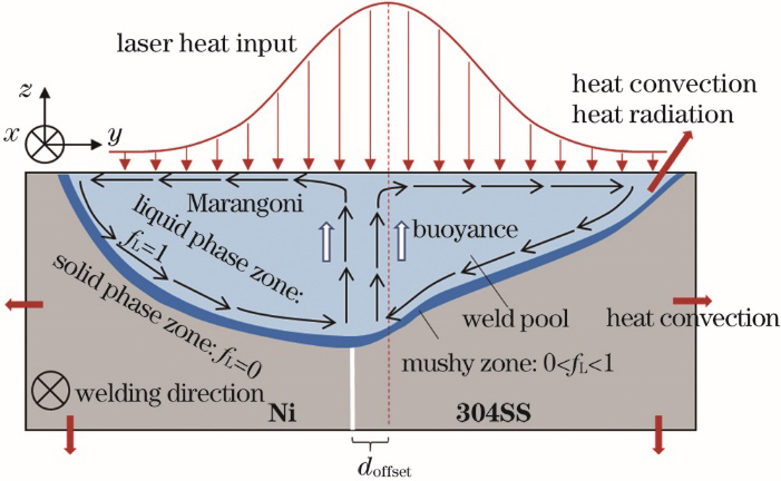
Fig. 1. Schematic diagram of the laser welding of dissimilar metals
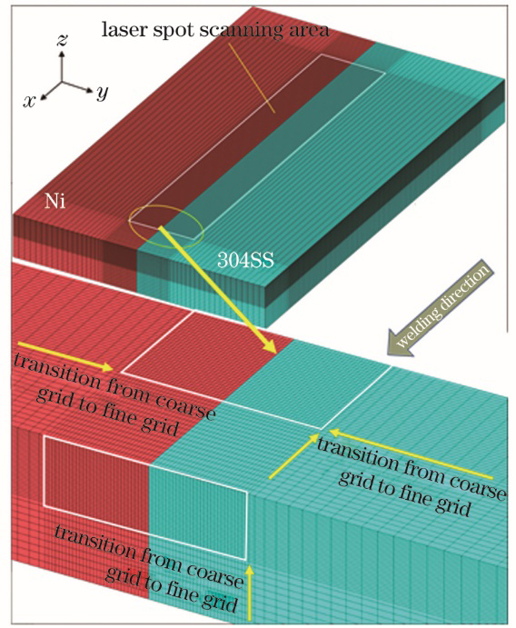
Fig. 2. Schematic diagram of the calculation model
Fig. 3. Cross-section of the molten pool. (a) Simulation result; (b) experimental result
Fig. 4. Calculation and experimental results of the element distribution
Fig. 5. Evolution of the molten pool. (a) Geometry profile and the distribution of Fe elements on the top surface; (b) geometric dimensions
Fig. 6. Distribution of Fe elements and liquid velocity on the cross section of the molten pool. (a) Relative position of the cross section; (b) plane 1; (c) plane 2; (d) plane 3
Fig. 7. Orthogonal simulation results of the process parameter correlation
Fig. 8. Mass fraction of Fe element in the longitudinal section. (a) Vscan=10 mm/s; (b) Vscan=20 mm/s; (c) Vscan=30 mm/s
Fig. 9. Mass fraction of Fe element under different offsets. (a) Longitudinal section; (b) cross section
Fig. 10. Distribution of Fe element under different parameters. (a) Parameters before adjustment; (b) parameters after adjustment
|
Table 1. Mass fraction of elements in 304SS material unit: %
| |||||||||||||||||||||||||||||
Table 2. Design of orthogonal parameters
|
Table 3. Experimental results of the orthogonal simulation
|
Table 4. Range analysis results
|
Table 5. Mixing time the molten pool at different scanning velocity

Set citation alerts for the article
Please enter your email address
© Copyright 2018-2021 | Chinese Laser Press. All Rights Reserved 沪ICP备15018463号-20