Deterministic all-optical quantum state sharing

Yingxuan Chen; Qiqi Zhu; Xutong Wang; Yanbo Lou; Shengshuai Liu; Jietai Jing

doi:10.1117/1.AP.5.2.026006

Abstract

Quantum state sharing, an important protocol in quantum information, can enable secure state distribution and reconstruction when part of the information is lost. In (k, n) threshold quantum state sharing, the secret state is encoded into n shares and then distributed to n players. The secret state can be reconstructed by any k players (k > n / 2), while the rest of the players get nothing. In the continuous variable regime, the implementation of quantum state sharing needs the feedforward technique, which involves optic-electro and electro-optic conversions. These conversions limit the bandwidth of the quantum state sharing. Here, to avoid the optic-electro and electro-optic conversions, we experimentally demonstrate (2, 3) threshold deterministic all-optical quantum state sharing. A low-noise phase-insensitive amplifier based on the four-wave mixing process is utilized to replace the feedforward technique. We experimentally demonstrate that any two of three players can cooperate to implement the reconstruction of the secret state, while the rest of the players cannot get any information. Our results provide an all-optical platform to implement arbitrary (k, n) threshold deterministic all-optical quantum state sharing and pave the way to construct the all-optical broadband quantum network.

Keywords

four-wave mixing quantum information quantum state sharing

1 Introduction

Quantum information,1 which utilizes the laws of quantum mechanics to process and communicate information, is one of the key directions in quantum physics. Due to the introduction of the quantum effect, quantum information processing greatly improves the capacity of information processing and the security of communication. Therefore, quantum information has attracted extensive attention all over the world. In quantum information, discrete variable (DV)2 and continuous variable (CV)3 systems are two important platforms. In the DV system, the physical quantity that has a discrete spectrum is used to describe the quantum state, such as polarization and orbital angular momentum. The DV system has the advantage of being insensitive to losses.2 In contrast, in the CV system, the quantum state is described by the physical quantity that has a continuous spectrum, such as amplitude quadrature and phase quadrature. The CV system has the advantage of deterministic implementation.3 With the development of quantum technology, a series of quantum information protocols based on DV and CV systems have been developed, including quantum key distribution,4^,5 quantum teleportation,6^–14 entanglement swapping,15^–21 quantum dense coding,22^–27 quantum cloning,28^–32 and so on.

Among them, quantum state sharing (QSS), which enables secure state distribution and reconstruction, is an important quantum information protocol for constructing a quantum network. In this protocol, the dealer encodes a secret state into $n$ shares and distributes them to $n$ players. Any $k$ players ( $k > n / 2$ ) can cooperate to reconstruct the secret state, while the rest of the $n - k$ players get nothing. Due to this feature, QSS can be used in quantum error correction in which up to $n - k$ nodes malfunction.33 QSS can also be utilized in the construction of scalable quantum information networks, the transmission of entanglement over faulty channels, and the implementation of multipartite quantum cryptography.33 The QSS was first proposed in the DV regime.34^,35 Then, such protocol was transplanted to the CV regime.36 In the CV regime, the (2, 3) threshold deterministic QSS has been studied both in theory37 and experiment.37^,38 However, the feedforward technique is needed for implementing QSS in the CV regime.38 The feedforward technique involves the optic-electro and electro-optic conversions, which limits the bandwidth of QSS. Therefore, to broaden the bandwidth of QSS, optic-electro and electro-optic conversions should be avoided.

In CV regime, all-optical QSS (AOQSS) based on a phase-insensitive amplifier (PIA), which avoids the feedforward technique in QSS, has been theoretically proposed.37 However, it is difficult to directly control the inherent noise coupled into the amplified output state of PIA.37 Therefore, such AOQSS has never been experimentally implemented. Here, we experimentally demonstrate (2, 3) threshold deterministic AOQSS by utilizing a low-noise PIA based on a double- $Λ$ configuration four-wave mixing (FWM) process.39^–44 We encode the secret state into three shares and distribute them to three players. We demonstrate that any two players can cooperate to retrieve the secret state, while the rest of the players get nothing. The average fidelity of all reconstruction structures is $0.74 \pm 0.02$ , which beats the corresponding classical limit of 2/3.

Sign up for Advanced Photonics TOC. Get the latest issue of Advanced Photonics delivered right to you！Sign up now

2 Results

2.1 Principle of AOQSS and Experimental Setup

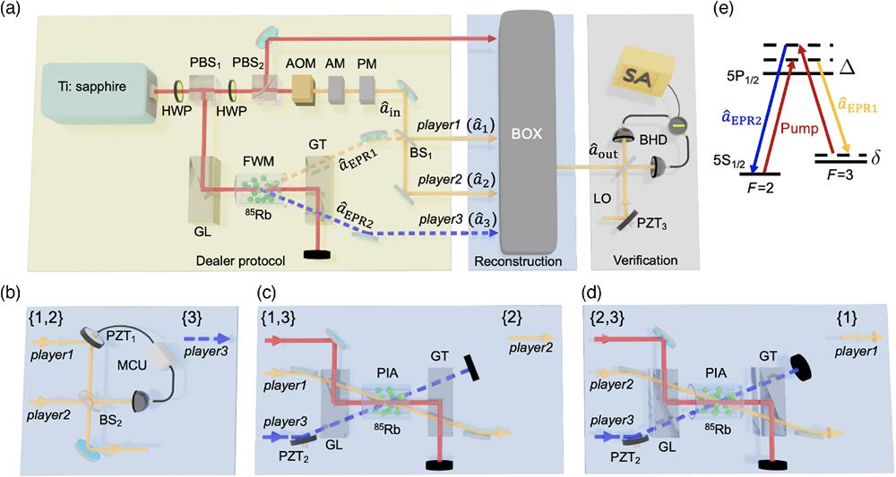
The experimental setup of the deterministic AOQSS protocol is shown in Fig. 1. The Ti:sapphire laser, whose frequency is about 1 GHz blue detuned from the $D 1$ line ( $5 S_{1 / 2}, F = 2 \to 5 P_{1 / 2}$ , 795 nm) of ${}^{85}{Rb}$ , is divided into two by a polarization beam splitter ( ${PBS}_{1}$ ). The vertically polarized one with a power of about 100 mW serves as the pump beam for generating Einstein–Podolsky–Rosen (EPR) entangled source45 based on the FWM process.39^–44 Its waist is about $650 μ m$ at the center of a 12-mm long hot ${}^{85}{Rb}$ vapor cell whose temperature is stabilized at around 116.5°C. The Hamiltonian of the FWM process is given as44 $\hat{H} = i ℏ r {\hat{a}}_{EPR 1}^{†} {\hat{a}}_{EPR 2}^{†} + H . c .,$ (1)where ${\hat{a}}_{EPR 1}^{†}$ and ${\hat{a}}_{EPR 2}^{†}$ are the creation operators associated with EPR1 and EPR2, respectively. $r$ denotes the interaction strength of the FWM process. H.c. is the Hermitian conjugate. The output fields of the FWM process can be expressed as44 ${\hat{a}}_{EPR 1} (τ) = \sqrt{G_{1}} {\hat{a}}_{01} + \sqrt{G_{1} - 1} {\hat{a}}_{02}^{†}, {\hat{a}}_{EPR 2}^{†} (τ) = \sqrt{G_{1} - 1} {\hat{a}}_{01} + \sqrt{G_{1}} {\hat{a}}_{02}^{†},$ (2)where ${\hat{a}}_{01}$ , ${\hat{a}}_{02}$ are the annihilation operators of the vacuum input states. $G_{1} = \cosh^{2} (r τ)$ is the intensity gain of the FWM process, and $τ$ is the interaction time. As shown in Fig. 1(e), in this FWM process, two pump photons convert to one ${\hat{a}}_{EPR 1}$ photon, which is red-detuned by 3.04 GHz from the pump beam, and one ${\hat{a}}_{EPR 2}$ photon, which is blue-detuned by 3.04 GHz from the pump beam. The horizontally polarized one from ${PBS}_{1}$ is further divided into two beams by ${PBS}_{2}$ . To generate the secret coherent state ${\hat{a}}_{in}$ , which is redshifted by 3.04 GHz from the pump beam, we pass the weak one from ${PBS}_{2}$ through an acousto-optic modulator. Then, classical amplitude and phase signals are encoded on the secret beam through an amplitude modulator (AM) and a phase modulator (PM), respectively. After that, ${\hat{a}}_{in}$ and ${\hat{a}}_{EPR 1}$ are combined by a beam splitter ( ${BS}_{1}$ ) whose transmittance is $1 / 2$ . The two outputs ${\hat{a}}_{1}$ and ${\hat{a}}_{2}$ are sent to player1 and player2, respectively. ${\hat{a}}_{EPR 2}$ is sent to player3 and denoted as ${\hat{a}}_{3}$ . To further enhance the security of the AOQSS protocol, additional Gaussian noise is encoded onto the three shares, which can be expressed as38 ${\hat{a}}_{1} = ({\hat{a}}_{in} - {\hat{a}}_{EPR 1} - δ N) / \sqrt{2}, {\hat{a}}_{2} = ({\hat{a}}_{in} + {\hat{a}}_{EPR 1} + δ N) / \sqrt{2}, {\hat{a}}_{3} = {\hat{a}}_{EPR 2} + δ N^{*} .$ (3)

$The detailed experimental setup of the deterministic AOQSS protocol. (a) The detailed experimental scheme. (b) {1,2} reconstruction structure. (c) {1,3} reconstruction structure. (d) {2,3} reconstruction structure. HWP, half-wave plate; GL, Glan–laser polarizer; GT, Glan–Thompson polarizer; a^in, the annihilation operator associated with the secret coherent state; a^1, a^2, and a^3, the annihilation operators associated with three shares held by player1, player2, and player3, respectively. (e) Energy level diagram of the double-Λ scheme in the D1 line of Rb85. Δ, one-photon detuning; δ, two-photon detuning.$

Figure 1.The detailed experimental setup of the deterministic AOQSS protocol. (a) The detailed experimental scheme. (b) ${1,2}$ reconstruction structure. (c) ${1,3}$ reconstruction structure. (d) ${2,3}$ reconstruction structure. HWP, half-wave plate; GL, Glan–laser polarizer; GT, Glan–Thompson polarizer; ${\hat{a}}_{in}$ , the annihilation operator associated with the secret coherent state; ${\hat{a}}_{1}$ , ${\hat{a}}_{2}$ , and ${\hat{a}}_{3}$ , the annihilation operators associated with three shares held by player1, player2, and player3, respectively. (e) Energy level diagram of the double- $Λ$ scheme in the $D 1$ line of ${}^{85}{Rb}$ . $Δ$ , one-photon detuning; $δ$ , two-photon detuning.

The additional Gaussian noise is denoted by $δ N = ({\hat{X}}_{N} + i {\hat{Y}}_{N}) / 2$ , which has a mean of $⟨ {\hat{X}}_{N} ⟩ = ⟨ {\hat{Y}}_{N} ⟩ = 0$ and variance of $Δ^{2} {\hat{X}}_{N} = Δ^{2} {\hat{Y}}_{N} = V_{N}$ . The $\hat{X}$ ( $\hat{X} = {\hat{a}}^{†} + \hat{a}$ ) and $\hat{Y}$ ( $\hat{Y} = i {\hat{a}}^{†} - i \hat{a}$ ) are the amplitude quadrature and phase quadrature of the state, respectively. Note that the additional Gaussian noise is introduced naturally in our EPR generation process. (See Sec. 1 of the Supplemental Material for the noise power spectra of ${\hat{a}}_{in}$ , ${\hat{a}}_{1}$ , ${\hat{a}}_{2}$ , and ${\hat{a}}_{3}$ .)

For the (2, 3) threshold deterministic AOQSS protocol, there are three different reconstruction protocols. In this sense, we send these shares into three reconstruction boxes, which are indicated by Figs. 1(b)–1(d) for ${1,2}$ , ${1,3}$ , and ${2,3}$ structures, respectively. For the ${1,2}$ reconstruction structure shown in Fig. 1(b), ${\hat{a}}_{1}$ and ${\hat{a}}_{2}$ are combined with $50 : 50 {BS}_{2}$ . The piezoelectric transducer ( ${PZT}_{1}$ ) placed in the path of ${\hat{a}}_{1}$ is used to change the relative phase between ${\hat{a}}_{1}$ and ${\hat{a}}_{2}$ . After locking the relative phase between ${\hat{a}}_{1}$ and ${\hat{a}}_{2}$ with a microcontrol unit,46 the ${BS}_{2}$ has one bright output and one vacuum output. The bright output is the reconstructed state of the ${1,2}$ structure. The quadratures of the output reconstructed state ${\hat{a}}_{out}$ can be expressed as37 ${\hat{X}}_{out} = \frac{{\hat{X}}_{1} + {\hat{X}}_{2}}{\sqrt{2}} = {\hat{X}}_{in}, {\hat{Y}}_{out} = \frac{{\hat{Y}}_{1} + {\hat{Y}}_{2}}{\sqrt{2}} = {\hat{Y}}_{in} .$ (4)

It can be seen that the ${1,2}$ structure can completely reconstruct the secret state. ${3}$ is the corresponding adversary structure, in which ${\hat{a}}_{3}$ carries no information on the secret state.

For the ${1,3}$ structure, the secret state reconstruction is implemented by amplifying ${\hat{a}}_{1}$ with the help of ${\hat{a}}_{3}$ in a PIA based on the FWM process. As shown in Fig. 1(c), the strong one from ${PBS}_{2}$ serves as the pump for the PIA. It crosses with ${\hat{a}}_{1}$ and ${\hat{a}}_{3}$ symmetrically at the center of the second 12-mm long ${}^{85}{Rb}$ vapor cell, whose temperature is stabilized at 118°C. The angle between ${\hat{a}}_{3}$ and the pump beam is about 7 mrad. The ${PZT}_{2}$ placed in the path of ${\hat{a}}_{3}$ is used to change the relative phase between ${\hat{a}}_{1}$ and ${\hat{a}}_{3}$ . ${2}$ is the corresponding adversary structure. When the intensity gain of the PIA ( $G_{2}$ ) is set to 2, the quadratures of the output reconstructed state ${\hat{a}}_{out}$ can be expressed as ${\hat{X}}_{out} = {\hat{X}}_{in} + {\hat{X}}_{EPR 2} - {\hat{X}}_{EPR 1}, {\hat{Y}}_{out} = {\hat{Y}}_{in} - {\hat{Y}}_{EPR 2} - {\hat{Y}}_{EPR 1} .$ (5)

The ${2,3}$ structure is equivalent to the ${1,3}$ structure in the (2, 3) threshold QSS.38 The ${2,3}$ structure is shown in Fig. 1(d). ${1}$ is the corresponding adversary structure. It can be seen that the functions of PIA are coupling the quadratures of ${\hat{a}}_{3}$ into the output state and reaching the unity gain point when the gain of PIA is set to 2. In other words, the physical essence of this PIA is reconstructing the secret state.

To quantify the quality of the reconstructed state of deterministic AOQSS protocol, we utilize its fidelity $F$ , which is defined as $F = ⟨ Ψ_{in} | ρ_{out} | Ψ_{in} ⟩$ .47 Assuming that all states involved are Gaussian and the secret state is a coherent state, the fidelity can be expressed as37^,38 $F = 2 e^{- (k_{x} + k_{y}) / 4} / \sqrt{(1 + Δ^{2} {\hat{X}}_{out}) (1 + Δ^{2} {\hat{Y}}_{out})},$ (6)where $k_{x} = {⟨ {\hat{X}}_{in} ⟩}^{2} {(1 - g_{x})}^{2} / (1 + Δ^{2} {\hat{X}}_{out})$ , $k_{y} = {⟨ {\hat{Y}}_{in} ⟩}^{2} {(1 - g_{y})}^{2} / (1 + Δ^{2} {\hat{Y}}_{out})$ , $g_{x} = ⟨ {\hat{X}}_{out} ⟩ / ⟨ {\hat{X}}_{in} ⟩$ , and $g_{y} = ⟨ {\hat{Y}}_{out} ⟩ / ⟨ {\hat{Y}}_{in} ⟩$ . Without the help of the EPR entangled source, the maximum achievable fidelities of ${1,2}, {1,3}$ , and ${2,3}$ reconstruction structures are $F_{{1,2}}^{clas} = 1, F_{{1,3}}^{clas} = 1 / 2$ , and $F_{{2,3}}^{clas} = 1 / 2$ , respectively. Therefore, the classical fidelity limit of the (2, 3) threshold AOQSS protocol is $F_{avg}^{clas} = \frac{F_{{1,2}}^{clas} + F_{{1,3}}^{clas} + F_{{2,3}}^{clas}}{3} = 2 / 3$ (See Sec. 2 of the Supplemental Material for a detailed derivation). If the average fidelity is higher than the classical limit of AOQSS, the AOQSS succeeds.

To check the performance of the AOQSS, the reconstructed state ${\hat{a}}_{out}$ is measured by a balanced homodyne detection (BHD). The local oscillator (LO) is obtained by setting up a similar bright-seed setup, which is a few millimeters above the current beams. The relative phase between ${\hat{a}}_{out}$ and LO is changed by ${PZT}_{3}$ . The transimpedance gain of the balanced detector is $10^{5} V / A$ , and the quantum efficiency of balanced detector is about 97%. The variances of the amplitude (locking the phase of BHD to 0) and phase (locking the phase of BHD to $π / 2$ ) quadratures of ${\hat{a}}_{out}$ are analyzed by a spectrum analyzer (SA).

2.2 Experimental Results and Discussion

Figure 2 shows the typical noise power results for ${1,2}$ reconstruction structure. As shown in Figs. 2(a) and 2(b), the blue dashed traces (orange solid traces) are the measured variances of amplitude quadrature and phase quadrature of ${\hat{a}}_{in}$ ( ${\hat{a}}_{out}$ ) with modulation signals at 1.5 MHz. The overlap between the modulation signal peaks of ${\hat{a}}_{in}$ and ${\hat{a}}_{out}$ shows that the input state ${\hat{a}}_{in}$ and output state ${\hat{a}}_{out}$ have the same amplitude ( $g_{x}$ and $g_{y}$ are almost 1). To quantify the fidelity of ${1,2}$ reconstruction structure, we turn off the modulation signals of the secret state and measure the amplitude and phase quadrature variances for the input secret state ${\hat{a}}_{in}$ (blue traces) and the reconstructed output state ${\hat{a}}_{out}$ (orange traces), as shown in Figs. 2(c) and 2(d), respectively. The corresponding fidelity of the ${1,2}$ reconstruction structure is $F_{{1,2}} = 0.99 \pm 0.01$ . This means that we almost retrieve the secret state, which is consistent with the theory.

Figure 2.The typical noise power results for ${1,2}$ reconstruction structure. (a) and (b) The amplitude and phase quadrature variances with classical modulations for the input secret state (blue dashed traces) and the output state (orange solid traces), respectively. (c) and (d) The amplitude and phase quadrature variances without classical modulations for the input secret state (blue traces) and the output state (orange traces) at 1.5 MHz, respectively. The vertical scale is normalized to the quadrature variances of the input secret state.

The typical noise power results for the deterministic AOQSS with ${1,3}$ reconstruction structure are shown in Fig. 3. The noise spectra with modulations for amplitude and phase quadratures are shown in Figs. 3(a) and 3(b), respectively. The blue dashed trace in Figs. 3(a) and 3(b) shows the amplitude (phase) quadrature variance of the input state. The amplitude (phase) quadrature variance of the output state without the EPR entangled source is represented by the orange solid trace in Figs. 3(a) and 3(b). The overlap of the peaks on the blue dashed traces and the orange solid traces shows that the gains $g_{x}$ and $g_{y}$ of the ${1,3}$ reconstruction structure are almost unity. To quantify the fidelity of the AOQSS with the ${1,3}$ reconstruction structure, we also turn off the modulation signals and measure the amplitude and phase quadrature variances for the input secret state ${\hat{a}}_{in}$ and the reconstructed output state ${\hat{a}}_{out}$ , as shown in Figs. 3(c) and 3(d), respectively. In Figs. 3(c) and 3(d), the blue traces show the amplitude and phase quadrature variances of the input secret state, respectively. With the help of the entangled source, the variances of the amplitude and phase quadratures of ${\hat{a}}_{out}$ are shown as the green traces in Figs. 3(c) and 3(d), respectively. The relative phase between the two EPR entangled beams is scanned by ${PZT}_{2}$ . When the variance of the amplitude (phase) quadrature of the output state reaches the minima of the green trace in Figs. 3(c) and 3(d), the relative phase between ${\hat{a}}_{EPR 1}$ and ${\hat{a}}_{EPR 2}$ corresponds to ${\hat{X}}_{EPR 2} - {\hat{X}}_{EPR 1}$ ( ${\hat{Y}}_{EPR 2} + {\hat{Y}}_{EPR 1}$ ). Therefore, we can treat the minima of green traces in Figs. 3(c) and 3(d) as the variances of ${\hat{X}}_{out}$ and ${\hat{Y}}_{out}$ of the reconstructed output state, respectively. Consequently, the fidelity of the AOQSS with the ${1,3}$ structure is $F_{{1,3}} = 0.62 \pm 0.02$ , as the variances of ${\hat{X}}_{out}$ and ${\hat{Y}}_{out}$ are $3.50 \pm 0.21 dB$ and $3.46 \pm 0.20 dB$ above the corresponding variances of ${\hat{X}}_{in}$ and ${\hat{Y}}_{in}$ , respectively. The orange traces show the variances of the output state without the help of the EPR entangled source, which are referred to the corresponding classical ${1,3}$ structure. We can see that, without the EPR entangled source, the amplitude (phase) variance of the output state is $4.86 \pm 0.12 dB$ ( $4.81 \pm 0.11 dB$ ) above the input state ${\hat{a}}_{in}$ . It can be calculated that the fidelity of the classical ${1,3}$ structure (corresponding classical limit) is $0.49 \pm 0.01$ . Figures 3(e) and 3(f) show the noise spectra for the adversary structure ${2}$ . The peaks of orange traces (quadrature variances of ${\hat{a}}_{2}$ with modulation) are about 3 dB below the peak of the blue traces (quadrature variances of ${\hat{a}}_{in}$ with modulation), which means that $g_{x}$ and $g_{y}$ are almost $\sqrt{1 / 2}$ . Then, based on the red traces (quadrature variances of ${\hat{a}}_{2}$ without modulation) and the black traces (quadrature variances of ${\hat{a}}_{in}$ without modulation) in Figs. 3(e) and 3(f), the obtained fidelity for the ${2}$ structure is only $F_{{2}} = 0.09 \pm 0.01$ . In other words, player2 gets almost nothing. The typical results for the AOQSS with a ${2,3}$ reconstruction structure are shown in the Sec. 3 of the Supplemental Material, which are similar to Fig. 3. The obtained fidelity for the AOQSS with a ${2,3}$ structure is $F_{{2,3}} = 0.61 \pm 0.02$ . In this sense, the average fidelity for the (2, 3) threshold deterministic AOQSS is $F_{avg} = 0.74 \pm 0.02$ , which beats the corresponding theoretical (experimental) classical limit of 2/3 (about 0.66). In other words, we successfully experimentally implement the (2, 3) threshold deterministic AOQSS. It is worth noting that the reconstructed state of our AOQSS is in the same form as the secret state, which is distinct from the experiments in Refs. [37] and [38], whose reconstructed state has a different form from the secret state. This results in the directly measured fidelity of the experiments in Refs. [37] and [38] being very low, and a posteriori must be applied to the reconstructed state to obtain a meaningful fidelity. Therefore, our AOQSS without a posteriori is essentially different from the experiments in Refs. [37] and [38].

Figure 3.The typical noise power results for ${1,3}$ reconstruction structure and the corresponding adversary structure ${2}$ . (a) and (b) The amplitude and phase quadrature variances with classical modulations for the input secret state (blue dashed traces) and the output state (orange solid traces) of the classical ${1,3}$ structure, respectively. (c) and (d) The amplitude and phase quadrature variances without the classical modulations for the input secret state (blue traces), the output state of ${1,3}$ structure (green traces), and the corresponding classical ${1,3}$ structure (orange traces), respectively. The center frequency of SA is set to 1.5 MHz. (e) and (f) The amplitude and phase quadrature variances of ${2}$ structure, respectively. The input secret state and the output state with (without) classical modulations are shown as the blue (black) traces and the orange (red) traces, respectively. The vertical scale is normalized to the quadrature variances of the input secret state.

To show the advantage of our deterministic AOQSS protocol, which avoids the optic-electro and electro-optic conversions, we scan the analysis frequency from 1.4 to 2.4 MHz and measure the fidelities for AOQSS with the ${1,3}$ structure, as shown in Fig. 4. The fidelity of AOQSS versus analysis frequency is shown as the blue trace, while the corresponding classical limit is shown as the orange trace. It can be seen that as the analysis frequency ranges from 1.4 to 2.4 MHz, the fidelities of AOQSS with the ${1,3}$ structure can beat the corresponding classical limit, which shows that the AOQSS can be successfully implemented within this sideband frequency range. When the analysis frequency is larger than 2 MHz, the slight decrease of fidelity is due to the decrease of the squeezing of the EPR entangled source.

Figure 4.The experimental fidelities versus the sideband frequency. The fidelities of deterministic AOQSS with a ${1,3}$ reconstruction structure and corresponding experimental classical limit are shown as the blue trace and the orange trace, respectively. The error bars are obtained from the standard deviations of multiple repeated measurements.

To implement a scaled-up version of the (2, 3) threshold deterministic AOQSS, there is no need to increase the number of active elements (PIAs) required by the players for retrieving the secret state, while the number of EPR entangled sources (two-mode squeezed states) required by the dealer should be increased.37^,48 In other words, in a scaled-up AOQSS, the dealer uses more EPR entangled sources and more passive elements (BSs) to encode a secret state. Correspondingly, a PIA and more passive elements (BSs) are utilized to retrieve the secret state. For example, a (3, 5) threshold deterministic AOQSS can be implemented by increasing one set of EPR entanglements and some passive elements, as shown in Sec. 4 of the Supplemental Material.

3 Conclusion

We have experimentally implemented a (2, 3) threshold deterministic AOQSS without a posteriori and the optic-electro and electro-optic conversions. We demonstrate that any two players can cooperate to retrieve the secret state, while the other player gets nothing. The average fidelity of all reconstruction structures is $0.74 \pm 0.02$ . More importantly, we have shown that AOQSS can be successfully implemented for the bandwidth ranging from 1.4 to 2.4 MHz. Our results provide a promising scheme to construct an all-optical broadband multipartite quantum network.

Yingxuan Chen is a PhD candidate in optics at the State Key Laboratory of Precision Spectroscopy, East China Normal University under the supervision of Professor Jietai Jing. Her current research interests include quantum optics and quantum information, especially quantum communication protocols.

Qiqi Zhu is a PhD candidate in optics at the State Key Laboratory of Precision Spectroscopy, East China Normal University under the supervision of Professor Jietai Jing. His current research interests include quantum optics and quantum communication.

Xutong Wang is a PhD candidate in optics at the State Key Laboratory of Precision Spectroscopy, East China Normal University under the supervision of Professor Jietai Jing. His current research interests include quantum optics and quantum information, especially the generation and distribution of high-capacity and multi-beam quantum light sources.

Yanbo Lou is an associate professor at the State Key Laboratory of Precision Spectroscopy of East China Normal University, Shanghai, China. He received his PhD in optics from the East China Normal University in 2021. His current research interests include high-capacity quantum information protocols, high-precision quantum metrology, and high-resolution quantum imaging.

Shengshuai Liu is a young professor at the State Key Laboratory of Precision Spectroscopy of East China Normal University, Shanghai, China. He received his PhD in optics from the East China Normal University in 2020. His current research interests include the generation of high-quality quantum squeezing and their applications in quantum information.

Jietai Jing is a professor at the State Key Laboratory of Precision Spectroscopy of East China Normal University, Shanghai, China. He received his PhD in optics from the Shanxi University in 2004. He did his postdoctoral work at the University of Virginia and the University of Maryland, College Park. His main research field is quantum optics and quantum information, especially the generation of high-capacity, multi-beam, low-noise quantum light sources, and their applications in quantum information.

References

[1] A. Galindo, M. A. Martín-Delgado. Information and computation: classical and quantum aspects. Rev. Mod. Phys., 74, 347-423(2002).

[2] J.-W. Pan et al. Multiphoton entanglement and interferometry. Rev. Mod. Phys., 84, 777-838(2012).

[3] S. L. Braunstein, P. van Loock. Quantum information with continuous variables. Rev. Mod. Phys., 77, 513-577(2005).

[4] V. Scarani et al. The security of practical quantum key distribution. Rev. Mod. Phys., 81, 1301-1350(2009).

[5] F. Xu et al. Secure quantum key distribution with realistic devices. Rev. Mod. Phys., 92, 025002(2020).

[6] C. H. Bennett et al. Teleporting an unknown quantum state via dual classical and Einstein–Podolsky–Rosen channels. Phys. Rev. Lett., 70, 1895-1899(1993).

[7] D. Bouwmeester et al. Experimental quantum teleportation. Nature, 390, 575-579(1997).

[8] S. L. Braunstein, H. J. Kimble. Teleportation of continuous quantum variables. Phys. Rev. Lett., 80, 869-872(1998).

[9] A. Furusawa et al. Unconditional quantum teleportation. Science, 282, 706-709(1998).

[10] M. Riebe et al. Deterministic quantum teleportation with atoms. Nature, 429, 734-737(2004).

[11] S. Olmschenk et al. Quantum teleportation between distant matter qubits. Science, 323, 486-489(2009).