Off-axis parabolic (OAP) mirrors have now become an essential tool to focus ultrashort laser pulses down to micrometre size spots, thus allowing relativistic intensities () to be reached. Indeed, focusing by means of OAP, which basically enables to get rid of the nonlinear and dispersive effects occurring in refractive optics, is currently pursued on basically all of the 10 TW–1 PW scale laser facilities worldwide (see Ref. [1] for instance and references therein), providing intensities on target up to . The usage of OAP is also envisaged as essential to get tight focusing of the next generation scale lasers in order to reach an intensity on target in the range, thus allowing strong field quantum electrodynamics (QED) phenomena such as radiation reaction, vacuum polarization and pair production to be investigated^{[2, 3]}.

On the other hand, the wealth of physical processes involved in laser–matter interaction at relativistic or ultra-relativistic intensity requires a detailed knowledge of the spatial and temporal structure of the electromagnetic field in the focal region. For instance, laser–plasma interaction processes depending on the laser polarization, such as, among others, the ones involved in proton acceleration, via either target normal sheath acceleration or radiation pressure acceleration (see Refs. [4, 5] and references therein), or the excitation of parametric instabilities^[6–8], are normally modelled using focused pulses with an ideal space and time structure. The detailed study of the structure of the electromagnetic field of beams focused by means of parabolic surfaces was initially undertaken in the field of optical microscopy, and thus devoted to the investigation of on-axis reflecting parabolic surfaces. The earliest works were essentially based on geometric optics approaches^[9]; in Ref. [10] a mixed method is used, based on geometric propagation from the paraboloid surface to a spherical surface, which is then used, in turn, as a boundary surface for a vector diffraction treatment based on the Stratton–Chu^{[11, 12]} theory. The first studies based on a direct numerical integration of diffraction integrals, for either off-axis^[13] or on-axis^{[14, 15]} parabolic mirrors, date back to the early 2000s. Such approaches, made possible by the availability of advanced numerical integration schemes and increasingly powerful simulation platforms, were driven by the need for tight focusing in applications such as confocal microscopy (see Ref. [16] for instance). Beside theoretical/numerical studies^{[14, 15, 17]}, different focusing configurations were also experimentally investigated^[18–20].

Motivated by the widespread diffusion of OAP mirrors as optical devices to focus ultrashort laser pulses, a growing attention is being devoted by the community active in the field of ultraintense laser–matter interaction to the experimental characterization of the intensity pattern in the focal region of high-intensity beams. This is a crucial issue even in light of the strong wavefront aberrations which can be expected to occur in laser systems, unless wavefront correction techniques are applied. In particular, the available intensity in the focal plane has been studied for 100 TW scale systems both with^[21] and without^[22] correcting the wavefront distortions by means of adaptive mirrors. More recently, the study of the aberrations induced by a not ideal OAP alignment was undertaken from a theoretical as well as an experimental point of view^{[23, 24]}. In Ref. [24], in particular, a theoretical model was developed, based on a full vector diffraction treatment, to study parameters such as the maximum intensity and Strehl ratio in the focal region of an OAP in the presence of small misalignments. These parameters are of particular importance in the context of laser–matter interaction at ultrahigh intensity.

These latter studies did not account for the ultrashort duration of the pulse; in other words, no time dependence was considered. As it is known since the first works dealing with the focusing of ultrashort pulses by lenses^[25], the envelope of the focused pulse takes on a rather complex structure in the far-field region, so that analytical frameworks able to predict the detailed electromagnetic field behaviour of an ultrashort pulse focused by an OAP would be desirable. However, as it can be easily realized, such treatments are rather involved, due to both the ultrashort duration (also implying large bandwidth) and the structure of the boundary surface (that is, the reflecting OAP surface).

A theory enabling the study of the far field of femtosecond pulses focused by a parabolic mirror, although in an on-axis configuration, was recently presented in Ref. [26], aimed at investigating the ultimate intensity achievable under very tight focusing () with the next generation systems. In particular, the authors first develop a theoretical treatment based on vector diffraction theory for a monochromatic wave upon reflection from the on-axis parabolic surface; based on that, the fields in the focal region of a femtosecond pulse are then calculated using a coherent superposition of monochromatic beams with suitable spectral amplitude and phase relationships. A different approach was more recently proposed in Ref. [27]. The method provides an equation (for a hertz-type vector potential) with the same structure of a unidirectional pulse propagation equation, which can be thus numerically solved using standard beam propagation methods. The reflection from an on-axis parabolic surface is taken into account using suitable initial conditions for the beam to be propagated. By comparison with full vector diffraction calculations the authors find out that their method gives pretty accurate results down to , while a 2-step method, involving the numerical integration of a diffraction integral, has to be used for smaller numbers.

The works reported in Refs. [26, 27] both account for a time dependence of the focused ultrashort pulse at an envelope level. Recently, a group working in the field of terahertz radiation reported on an experiment in which the electric and magnetic fields of a THz beam focused with a OAP mirror were characterized with sub-cycle time resolution^{[28, 29]}. In particular, the authors observed a loss of the original polarization structure and the formation of what they call electromagnetic divergence and rotation at the time of the optical cycle at which the fields are supposed to vanish. In Ref. [28] the authors also develop a simple and approximate model; although not directly applicable to their experimental results, due to its validity strictly holding only for high numbers, this model predicts the observed loss of the original polarization. An approximate theoretical description of the electric field in the focal region has been also recently proposed by the same authors^[30]. Indeed, the first guess that the original beam polarization could not be preserved due to off-axis focusing dates back to Ref. [31], where a theoretical model is presented predicting that the polarization of a beam focused by an off-axis ellipsoidal mirror exhibits a (smooth) spatial dependence in the focal plane. However, this observation only concerned the time averaged pattern of the polarization direction and did not describe any change occurring at a sub-cycle level.

In this paper, we first present, in Section 2, an exact theoretical model allowing the electric and magnetic fields of a laser beam (with a super-Gaussian transverse profile) focused by an OAP to be calculated. Unlike previous works, our framework is based on a full vector diffraction treatment and also retains a time dependence of the fields as provided by their initial phases, thus allowing the electromagnetic field pattern to be retrieved at any given time within the optical cycle. Using this model and solving the resulting integrals by numerical calculations, we study then, in Section 3.1, the field maps at different times, showing that, as a result of the off-axis focusing, electric (magnetic) fields are generated, during the optical cycle, along directions different from the original polarization direction (or original magnetic field direction, respectively). In order to assess the importance of this unusual and unexpected effect, basically resulting in a generation of intra-cycle cross polarization, we carry out a parametric study as a function of the OAP number and focal length; we also show how this phenomenon depends upon the original pulse polarization direction with respect to the OAP geometry. Finally, in Section 4, after mentioning some possible consequences of this intra-cycle depolarization in the context of laser–plasma interaction, we draw some conclusions and outline some future work.

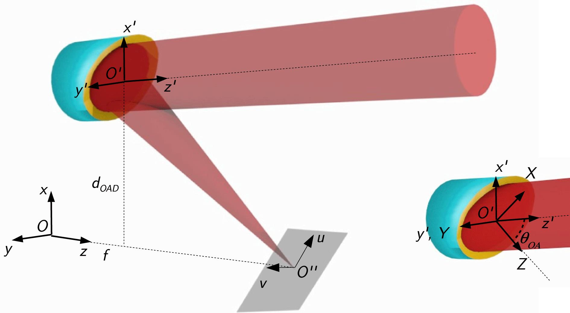
As typical in the field of ultrashort laser beam focusing, we consider in our model an OAP mirror whose boundary, projected onto a plane orthogonal to the (parent) paraboloid axis, is a circle. In other words, the mirror boundary results from the intersection of a revolution paraboloid surface and a cylinder with axis parallel to the paraboloid axis (we denote the distance between the two axes as ). The axis of the cylinder intersects the OAP surface at a point which from now on we will refer to as the ‘OAP centre’. Figure 1 provides some conventions used in the following. In particular, the system of Cartesian orthogonal coordinates is centred on the parent paraboloid vertex and is oriented in such a way that the parabola focus and the OAP centre ( in Figure 1) are located at the points , with , and , respectively. The meridional (sagittal) plane is thus the plane – (–). The OAP surface () is therefore identified by the equation

 (1)

We now consider a monochromatic beam, with a super-Gaussian transverse profile, incident along the direction; its electric and magnetic fields can thus be written, in the system, as

 (2)

 (3)

 (4)

We are now interested in the time-dependent behaviour of the electromagnetic fields in the focal region upon reflection off the OAP surface. As it is well known, the problem can be formally factorized into the time and space domains, and a suitable diffraction approach can be used to deal with this latter domain. As a consequence, we can write the field at the point at time as (a similar equation holds for ), where the spatial part has to be calculated using a suitable diffraction formulation; in our case, we use a full vector diffraction approach based on the Stratton–Chu theory (hence the subscript SC). As recently discussed in Ref. [32], the Stratton–Chu approach allows, generally speaking, beams with sharper transverse profiles to be dealt with, with respect to a more direct approach based on Green’s theorem applied to each field. It can be shown (see for instance our recent paper^[24]) that, assuming a perfect (100%) reflection, the boundary fields (on the OAP surface) appearing in the Stratton–Chu theory can be related to the incident fields, and the resulting integrals read

 (5)

 (6)

Using as parameters of the OAP surface just the coordinates of each point, we can write the (inward) normal to the surface as and the area element as . The incident fields in the above integrals must be expressed in the system and can be easily retrieved from equations (2) and (3); the electric field, for instance, can be written as . Here is the optical path from the point on the reference plane to the point on the OAP surface (notice that we are assuming ). The transverse field amplitude is obtained as .

On substituting all these expressions into equations (5) and (6) one thus gets, after some cumbersome algebra, the following equations for the (time-dependent) electric and magnetic field components focused by the OAP:

 (7)

 (8)

 (9)

 (10)

 (11)

 (12)

 (13)

 (14)

The real part of the fields, which we are going to use in the following, can be easily calculated from the above equations. In particular, it can be readily verified that

 (15)

 (16)

In the field of high-intensity laser–matter interaction, one is in general interested in the study of the field components along longitudinal and transverse directions with respect to the focused beam propagation direction, that is the direction along in Figure 1. With our conventions, this basically requires the knowledge of the field components in the system of coordinates ; it is readily verified that these components can be retrieved from the components in the system, provided by the integrals (15) and (16), using the obvious transformation , where is the matrix accounting for the rotation of an angle around the -axis.

In the following discussion, we use the coordinates and shown in Figure 1 to label the directions on a plane orthogonal to the central ray.

In this section, we discuss some general features of the electric and magnetic fields in the focal plane of the OAP, starting from a numerical integration of equations (15) and (16) at different times during the optical cycle. The numerical integration was performed using a multi-dimensional adaptive integration scheme based on the algorithm described in Ref. [33]. For the sake of the following discussion, we used a beam with and with a transverse amplitude profile given by formula (4) with and ; we also consider a rotationally symmetric beam () and set the value of so as to have a beam with an intensity full width at half-maximum (FWHM) of . The integration algorithm was implemented in a C code; with the above parameters, the integration required for each field component (at a given point and time) took typically a few hundreds of milliseconds to complete on a (Linux based) desktop PC equipped with a pretty standard CPU.

As said above, we are interested here in the field behaviour on the focal plane at different times of the optical cycle. For the sake of conciseness, from now on we will refer to the time at which the electric and magnetic fields at the centre of the observation plane (that is, at the point which the central ray is supposed to pass through) take on their maximum amplitude as ; conversely, we refer to the time at which both fields are supposed to vanish as .

The bottom right plot of Figure 2 (plot ) shows the direction and amplitude (normalized to 1) of the electric field (in the focal plane) at , for a beam polarized along ( in equations (2) and (3)) and focused by an OAP with and . As expected, the electric field is directed along the direction. The top right plot (plot ) shows, for the sake of a visual aid in considering the importance of the effects we are going to discuss, the intensity of the focused beam.

The first (left) column of Figure 2 shows the direction and amplitude of the electric (plot ) and magnetic (plot ) fields at . Here, a not obvious effect can be observed. Indeed, both the electric and magnetic fields actually only vanish in the surroundings of the central point, while a complex pattern is observed out of this point. Looking at the colour scale of these plots, one can see that the nonzero field components reach typical values of a few percent of those at ; we will discuss later how the importance of this effect depends upon the OAP parameters such as the number and the off-axis angle.

The middle column of Figure 2 shows the and field patterns at the other minimum within the optical cycle, that is at , being the radiation period. As it is rather predictable, the field patterns are similar to those encountered at , with the sign of the fields reversed.

It is interesting to look, at this point, at the behaviour of the fields for times very close to . Figure 3 shows the -field pattern for the times (top) and (bottom) (this time span corresponds to a few tens of attoseconds for a typical infrared laser beam). As it can be easily realized from this Figure, the region where the field actually vanishes does describe a sort of sweep along the meridional (–) plane. In other words, for a small neighbour of the points in the meridional plane, a time instant exists, close to , at which the field is zero; this time instant corresponds to only for the focal point.

The pattern of and is interchanged when an incident beam polarized along is considered; this can be seen in Figure 4, which shows the electric and magnetic field patterns at  for the same OAP and beam parameters as the ones considered in Figure 2 but with . Finally, as shown in Figure 5, the situation is somewhat intermediate for a beam incident on the OAP with a polarization at with respect to the – plane; in this case, the typical convergent/divergent pattern seen for the field (in the case ) or for the field (in the case ) is not encountered any more. However, it should be observed that the typical maximum amplitude of the fields at , which is of the order of a few percent of that at , does not depend on the beam polarization.

It is worth to observe that a longitudinal electric field component is also appearing at . Figure 6 shows a density map of the ratio of the longitudinal component to the transverse component , calculated at . As it can be realized by comparing with the top left plot of Figure 2, a longitudinal field component appears in the regions where the transverse field component is smaller (except for the neighbour of the central point).

Notice that in Figure 6 we have restricted our attention to a region of interest (ROI) over which the focused beam intensity keeps at a level greater than 0.1 of its maximum; in other words, we have only considered points such that and forced to a zero value all the points outside this ROI. Beside enabling a better readability of the plots, this procedure allows us to only consider a spatial region where the field observed at  has enough magnitude to potentially lead to nonnegligible physical effects in real laser–plasma interaction experiments. Unless otherwise specified, this procedure will be adopted in the following discussion.

We are now interested in investigating how the anomalous field patterns observed at the time  depend upon the OAP parameters, namely the number and the off-axis angle. To this purpose, we first look at the ratio of the square modulus of the electric field transverse component () at  to the corresponding quantity at . Notice that for this discussion, we restrict our attention to the field, since similar results obviously hold for the field.

Figure 7 shows the maps (restricted to the ROI defined above) of this ratio for an increasing off-axis angle (top row) and for an increasing number (bottom row). In particular, the top row shows the maps of for an OAP with (plot A) and (plot B). It can be seen that the amplitude of the field obtained at  is strongly dependent on the off-axis angle. In fact, by integrating the equations (15) and (16) for an on-axis parabola we find that the fields at  almost vanish across all the plane; the effects observed at  are thus a consequence of the off-axis focusing scheme. Analogously, the maps in the bottom row of Figure 7 show that the plays a role as well: tighter focusing causes larger field components to appear at .

As it is clear from Figure 7, the (relative) magnitude of the anomalous fields at  is not uniform across the ROI. For a quantitative assessment of the dependence upon the and of the observed phenomena, we thus need a spatially averaged quantity; we can consider, for instance, the integral of the square modulus of the transverse field averaged over the ROI using the local intensity as a weight:

 (1)

In particular, we define the parameter as the ratio of this quantity at  to the corresponding value at : . In Figure 8 we plot the parameters as a function of the off-axis angle (top) and of the number (bottom). Fitting the data, the following scaling laws can be obtained for the polarization:

 (17)

Starting from an exact time-dependent, vector diffraction based model developed on purpose, we have studied the electromagnetic field behaviour, at different times within the optical cycle, of a beam focused by an OAP mirror. In particular, we have investigated the electric and magnetic field patterns across planes orthogonal to the beam propagation direction.

A behaviour far from trivial was found, in the focal region, at the time () at which the electric and magnetic fields are supposed to vanish; actually, this zero field value only occurs in a small neighbour of the focus, while a complex electromagnetic field pattern exists at farther points. Such a complex pattern basically results in the appearance of field components orthogonal to the original polarization (or magnetic field) direction; furthermore, longitudinal field components (that is, directed along the original propagation direction) can also appear.

What seems to be relevant for laser–matter interaction experiments at relativistic intensities is the fact that the amplitude of these ‘anomalous’ electric and magnetic fields can reach, depending on the focusing conditions, values of a few percent of the maximum values expected during the optical cycle. Beside the boundaries of the beam, where the intensity (and thus the field amplitude) drops down to negligible values, this may occur, under some circumstances, even within a transverse spatial region where the field values are supposed to be high enough so as to potentially lead to nonnegligible effects on the laser–matter interaction dynamics.

As mentioned in the Introduction, such effects are to be possibly expected for laser–plasma interaction processes dependent on the laser polarization, in particular when tight focusing is employed, such as proton acceleration via either target normal sheath acceleration or radiation pressure acceleration. On the other hand, according to our results, the phenomena discussed in this paper are expected to be negligible at high numbers, so that, for instance, no departure from an ‘ideal’ laser beam is expected to occur in the context of Laser WakeField Acceleration experiments, where long focal length OAPs are commonly employed in order to sustain a long laser beam propagation.

As a final remark we observe that, in order to theoretically investigate possible effects in the laser–matter interaction at ultrahigh intensity, a full knowledge of the temporal dynamics of the field patterns discussed here would be needed. The discussion of a theory allowing such a study to be carried out is beyond the scope of the current paper and will be reported elsewhere. According to preliminary investigations carried out by numerically calculating the field integrals given above at different times close to the time  and studying the resulting patterns, we can estimate that the features observed around this time have typical timescales of the order of of the pulse cycle.

References

[1] C. Danson, D. Hillier, N. Hopps, D. Neely. High Power Laser Sci. Eng., 3, e3(2015).
[2] G. A. Mourou, T. Tajima, S. V. Bulanov. Rev. Mod. Phys., 78, 309(2006).
[3] A. Di Piazza, C. Müller, K. Z. Hatsagortsyan, C. H. Keitel. Rev. Mod. Phys., 84, 1177(2012).
[4] H. Daido, M. Nishiuki, A. S. Pirozhkov. Rep. Prog. Phys., 75(2012).
[5] A. Macchi, M. Borghesi, M. Passoni. Rev. Mod. Phys., 85, 751(2013).
[9] J. E. Howard. Appl. Opt., 18, 2714(1979).
[10] C. J. R. Sheppard, A. Choudhury, J. Gannaway. IEE J. Microwaves Opt. Acoust., 1, 129(1977).
[11] J. A. Stratton, L. J. Chu. Phys. Rev., 56, 99(1939).
[12] J. D. Jackson. Classical Electrodynamics(1998).
[13] P. Argujio, M. S. Scholl, G. Paez. Appl. Opt., 40, 2909(2001).
[14] P. Varga, P. Török. J. Opt. Soc. Am. A, 17, 2081(2000).
[15] P. Varga, P. Török. J. Opt. Soc. Am. A, 17, 2090(2000).
[16] M. A. Lieb, A. J. Meixner. Opt. Express, 8, 458(2001).
[17] A. April, M. Piché. Opt. Express, 18(2010).
[18] J. Stadler, C. Stanciu, C. Stupperich, A. J. Meixner. Opt. Lett., 33, 681(2008).
[19] A. Drechsler, M. A. Lieb, C. Debus, A. J. Meixner, G. Tarrach. Opt. Express, 9, 637(2001).
[20] R. Dorn, S. Quabis, G. Leuchs. Phys. Rev. Lett., 91(2003).
[23] R. Heathcote, R. J. Clarke, T. B. Winstone, J. S. Green. Proc. SPIE, 8844(2013).
[24] L. Labate, P. Ferrara, L. Fulgentini, L. A. Gizzi. Appl. Opt., 55, 6506(2016).
[25] M. Kempe, W. Rudolph. Phys. Rev. A, 48, 4721(1993).
[26] T. M. Jeong, S. Weber, B. Le Garrec, D. Margarone, T. Mocek, G. Korn. Opt. Express, 23(2015).
[28] K. Shibata, M. Takai, M. Uemoto, S. Watanabe. Phys. Rev. A, 92(2015).
[29] M. Takai, K. Shibata, M. Uemoto, S. Watanabe. Appl. Phys. Express, 9(2016).
[30] K. Shibata, M. Uemoto, M. Takai, S. Watanabe. J. Opt., 19(2017).
[31] J. A. Murphy. Int. J. Infrared Millimeter Waves, 8, 1165(1987).
[32] J. Peatross, M. Berrondo, D. Smith, M. Ware. Opt. Express, 25(2017).
[33] J. Bernsten, T. O. Espelid, A. Genz. ACM Trans. Math. Soft., 17, 437(1991).
Set citation alerts for the article
Please enter your email address
© Copyright 2018-2021 | Chinese Laser Press. All Rights Reserved 沪ICP备15018463号-20