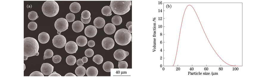
Fig. 1. AlMgScZr alloy powder. (a) Morphology of powder; (b) size distribution

Fig. 2. Relative densities of specimens fabricated under different scanning speeds

Fig. 3. Microstructures of longitudinal section of AlMgScZr alloy formed at 1200 mm/s scanning speed. (a) OM image; (b) SEM image

Fig. 4. TEM images of longitudinal section of AlMgScZr alloy formed at 1200 mm/s scanning speed. (a) Bright-field image; (b) local enlargement of Fig. 4(a); (c) precipitated phase in fine grain region and its corresponding HRTRM image and FFT image; (d) precipitated phase in coarse grain region and its corresponding HRTEM image and FFT image

Fig. 5.

IPFs and grain size distributions of different specimens. (a) (c) IPFs; (d) (f) grain size distributions

Fig. 6.

Grain boundary mappings and grain boundary misorientation angle distributions of different specimens. (a) (c) Grain boundary mappings; (d) (f) grain boundary misorientation angle distributions

Fig. 7. Potentiodynamic polarization curves for specimens #1, #2, #3 in NaCl solution with mass fraction of 3.5%

Fig. 8. EIS measurement results. (a) Nyquist plot; (b)(c) Bode plots; (d) equivalent circuit model

Fig. 9. Corrosion morphologies of specimens. (a) OM image of corrosion morphology; (b) SEM image of corrosion morphology of specimen #1; (c) SEM image of corrosion morphology of specimen #2; (d) SEM image of corrosion morphology of specimen #3

Table 1. Chemical compositions of AlMgScZr alloy

Table 2. Process parameters for SLM forming

Table 3. Fitting results corresponding to Fig. 7

Table 4. Fitting results corresponding to Fig. 8