• High Power Laser Science and Engineering
  • Vol. 8, Issue 3, 03000e28 (2020)
Lei Xia1、2, Yuanzhang Hu1, Wenyu Chen1, and Xiaoguang Li1、*
Author Affiliations
  • 1Institute for Advanced Study, Shenzhen University, Shenzhen 518060, China
  • 2Key Laboratory of Optoelectronic Devices and Systems of Ministry of Education and Guangdong Province, College of Optoelectronic Engineering, Shenzhen University, Shenzhen 518060, China
  • show less
    DOI: 10.1017/hpl.2020.29 Cite this Article Set citation alerts
    Lei Xia, Yuanzhang Hu, Wenyu Chen, Xiaoguang Li. Decoupling of the position and angular errors in laser pointing with a neural network method[J]. High Power Laser Science and Engineering, 2020, 8(3): 03000e28 Copy Citation Text show less

    Abstract

    In laser-pointing-related applications, when only the centroid of a laser spot is considered, then the position and angular errors of the laser beam are often coupled together. In this study, the decoupling of the position and angular errors is achieved from one single spot image by utilizing a neural network technique. In particular, the successful application of the neural network technique relies on novel experimental procedures, including using an appropriate small-focal-length lens and tilting the detector, to physically enlarge the contrast of different spots. This technique, with the corresponding new system design, may prove to be instructive in the future design of laser-pointing-related systems.

    1 Introduction

    Accurate laser pointing is crucial for many applications such as free-space communication[1], fusion ignition[2], high-power lasers[3] and robot manipulators[4]. The position and angular errors of a laser beam should therefore be accurately measured and synchronously adjusted. In measurements based on the centroidal position of a laser spot[57] the two errors are often coupled together, which means that they cannot be determined with one single measurement. The pure angular error in many applications can actually be obtained with the detector located on the in-focus plane. In this case, however, the position error of the laser is totally sacrificed. For applications requiring both the position and angular errors, such as fine optical systems[8], laser resonator alignment[9], laser beam drift control[10] and lithography[11,12], the common decoupling method for these two errors involves making two measurements, with one measurement on the in-focus plane and the other on the out-of-focus plane. It can be implemented by repositioning detectors at different locations[9], or splitting the beam into two paths[1014]. Since these methods only utilize information regarding spot centroids, long-focal-length lenses are required to improve the sensitivity of the spot centroid displacement. Optical measurement systems using these methods inevitably involve complex structures and a reduction in system reliability.

    The artificial neural network technique can establish the connection between the input and the output of systems by learning from datasets, and has been used in many fields for function approximation and pattern recognition[15,16]. In particular, this technique has already been used in many different optical systems. In adaptive optics systems, neural networks have been applied to derive the distorted wavefront from a simultaneous pair of in-focus and out-of-focus images of a reference star[1719]. Breitling et al. have used neural networks to predict the angular deviation of a pulse laser from the final four sample positions[20]. Guo et al. have utilized neural networks to reconstruct the wavefront of human eyes from the spot displacements from a Hartman–Shack sensor[21]. Abbasi et al. have adopted neural networks to obtain the position vector of a Gaussian beam for vibration analysis from four quad cell power distributions[22]. Yu et al. have employed neural networks to obtain the tilt, decenter and defocus of a laser diode fast-axis collimator from four parameters from the measured field distribution[23].

    In this study, a neural network is applied to extract full information from the intensity distribution of a laser spot, and the position and angular errors of a laser beam can be determined from a single spot image. The datasets for the neural network are obtained by the simulation of a prototype laser-pointing system with a special setup, including a tilted charge-coupled device (CCD) detector with known defocus distance and a small-focal-length lens. This setup is designed for obtaining spot images with more distinct features for neural network analysis, such as higher intensity contrast and the required spot size. Compared with traditional setups, the current system supplies a more compact structure and an alternative way to approach high measurement accuracy through data methods, so there may be some advantages in accuracy, reliability and synchronization in laser-pointing measurement.

    2 Neural network method for laser-pointing error measurement

    Our prototype laser-pointing system contains a laser source, a thin lens and a CCD detector, as shown in Figure 1. In the prototype system, for a beam tilt T the corresponding spot image M on the CCD is simulated through a virtual optical system method for a tilted beam[24]. The distance u between the source plane and the lens is set to be equal to the focal length f, so that the image beam waist can be approximately located on the focal plane for its largest waist radius ${w}_{02}\approx \lambda f/\left(\pi {w}_{01}\right)$ (half width at 1/e2 center intensity), and the spot radius w2 on the CCD can then be expressed as ${w}_2\approx {w}_{02}\sqrt{1+{\left({\delta}_z/{Z}_{R2}\right)}^2}$ , where ZR2 is the Rayleigh length in the image space, w01 is the waist radius at the source plane and λ is the wavelength of the laser source.

    We chose a laser of the wavelength λ = 632.8 nm, and a beam waist radius w01 = 2.0 mm with Gaussian distribution at the beam waist, corresponding to a typical transverse electromagnetic mode (TEM00) He-Ne laser source. The CCD had a pixel size of 0.0057 mm, with an output gray level of 12 bits, providing an intensity range 0–4095. The pixel intensities of an image are all integers to simulate analog-to-digital (A/D) conversion, which is equivalent to introducing a detection noise of less than 0.5. We limit the position offsets a0 and b0 within the range [−0.5, 0.5] mm, and the inclination angles θx and θy within [−25, 25] Ҽrad. To compare the prediction performance for image sets with different system parameters, the intensity of the collimated beam at the center of the CCD is fixed to a particular value by adjusting the intensity of the laser source. A dataset composed of 12,000 spot images of 36 × 36 pixel regions with the corresponding randomly generated beam tilts can then be obtained.

    Prototype laser-pointing system. S is the laser source; L is the thin lens; M is the spot image on the CCD; T is the beam tilt of the waist center on the source plane; a0, θx are the position offset and inclination angle of the beam relative to the optical axis in the x direction, respectively, and b0, θy are those in the y direction; u is the distance between the source plane and the lens; f is the focal length; δz is the defocus distance of the CCD. The optical axis of the system is along the z direction.

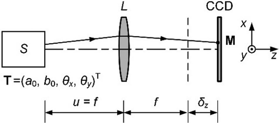
    Figure 1.Prototype laser-pointing system. S is the laser source; L is the thin lens; M is the spot image on the CCD; T is the beam tilt of the waist center on the source plane; a0, θx are the position offset and inclination angle of the beam relative to the optical axis in the x direction, respectively, and b0, θy are those in the y direction; u is the distance between the source plane and the lens; f is the focal length; δz is the defocus distance of the CCD. The optical axis of the system is along the z direction.

    The neural network used in this study is implemented by Python[25] without any specific package. It is a feed-forward network[19] with three layers: an input layer of 36 × 36 = 1296 nodes for normalized pixel intensities of an image, a hidden layer of 100 nodes and an output layer for the prediction of the normalized beam tilt. Samples from a dataset (10,000) are used to train the neural network for 2000 epochs with the back-propagation technique[26], and the remaining 2000 samples are used to test the performance of the neural network after each epoch of training. For the jth training epoch, the prediction error Ej of the neural network is evaluated as

    where an is the nth output of the network, yn is the nth actual beam tilt (normalized), m is the dimension of vector yn and N is the number of test samples. Finally, the mean value of Ej in the last 500 epochs of a total of 2000 epochs is employed to represent the prediction performance Emean of the neural network.

    Prediction errors Ej for all epochs, spot image M2 and image difference for beam tilts in the x direction. (a) and (b) show the prediction errors, the spot image and image difference on the vertical CCD, respectively. (c) and (d) show those on the tilted CCD with a rotation of 60° around the y-axis. (e) and (f) show those on the tilted CCD with a rotation of 60° around the x-axis.

    Figure 2.Prediction errors Ej for all epochs, spot image M2 and image difference for beam tilts in the x direction. (a) and (b) show the prediction errors, the spot image and image difference on the vertical CCD, respectively. (c) and (d) show those on the tilted CCD with a rotation of 60° around the y-axis. (e) and (f) show those on the tilted CCD with a rotation of 60° around the x-axis.

    In order to enlarge the image difference, we designed the system with a tilted CCD rotated by 60° around either the y or x axis. Figures 2(c) and 2(e) show the elliptical spots of image M2 with tilt T2 on the CCD rotated around the y and x axes, respectively. For the same beam tilts T1 and T2, the corresponding image differences are largely improved to −65.3 and 22.8 as shown in Figures 2(d) and 2(f), respectively. The significant enhancement can be attributed mainly to the magnified difference in incident angles and the no-longer centro-symmetric intensity distribution for the tilted CCD. As shown in the lower-left corner of Figure 2(d), since the incident angle of beam 2 is obviously larger than that of beam 1, the pattern for beam 2 exhibits a broader distribution with a lower peak value on the tilted CCD. For the pixels in Figure 2(f), the patterns of both beams deviate from the centro-symmetric distribution, giving the observed quadrupole image difference. The prediction results of the neural network are consistent with the changes in the image differences. As shown in Figures 2(c) and 2(e), the prediction performances Emean with the image rotation around the y and x axes are 0.010 and 0.014, respectively. It can therefore be inferred that the tilted CCDs can help to decouple the position and angular errors, and the rotation perpendicular to the beam tilt direction is better.

    For non-Gaussian beams, the maximum difference is expected to appear at different positions but with a similar magnitude. For flat-topped beams common in high-energy systems, the maximum difference would occur around the edges of the pattern with a similar magnitude; it is expected that this can be recognized accurately by a neural network, as discussed below.

    3 Results and discussion of prediction in two directions

    For practical prediction of beam tilts in two directions, we consider the prototype system under different combinations of parameters θ, f and δz. The tilting angle θ is chosen from 0°, 15°, 30°, 45° and 60°. The y = −x axis is chosen as the rotation axis of the CCD, allowing the spot to be stretched diagonally and contained in a smaller square pixel region. The focal length f is taken as 40, 60, 80, 100 or 120 mm. The spot images of the positive and negative defocus distances are symmetrical about the focal plane, so only the positive defocus distances δz/ZR2 = 0, 0.5, 1, 1.5 or 2 are considered. The positive defocus distance δz/ZR2 is set to a constant here, so that the spot radius can be changed with different focal length f. Finally, 125 generated datasets are substituted into the neural network to obtain the prediction performances of the beam tilts.

    Prediction performances Emean with different focal lengths f, tilting angles θ and defocus distances δz. (a) and (b) show spot samples and the prediction performance with typical focal lengths f = 40 and 100 mm, respectively. The partially enlarged plot in the dotted rectangle represents the prediction results for θ = 60°. (c) and (d) show the prediction performance when the tilting angles are 45° and 60°, respectively.

    Figure 3.Prediction performances Emean with different focal lengths f, tilting angles θ and defocus distances δz. (a) and (b) show spot samples and the prediction performance with typical focal lengths f = 40 and 100 mm, respectively. The partially enlarged plot in the dotted rectangle represents the prediction results for θ = 60°. (c) and (d) show the prediction performance when the tilting angles are 45° and 60°, respectively.

    To clearly elucidate the effect of the defocus distance, we focus on the prediction performances with the tilting angles θ =  45° and 60° as shown in Figures 3(c) and 3(d). In these cases, the factors that improve the neural network performance, such as larger spot size and image contrast, are competing with each other. A larger defocus distance can increase the spot size, but reduce other positive effects. For f ≥ 60 mm, the spot size may be sufficient for the network, and other factors play the leading role. Hence, the prediction performances deteriorate with the defocus distance. When f = 40 mm, the spot size is so small (5 × 5 for δz = 0, θ = 60° as shown in Figure 3(a)) that it plays a greater role in prediction. The two curves therefore show a downward trend, or zigzag downward.

    Similarly, we can derive the influence of the focal length from Figures 3(c) and 3(d). With a large defocus distance (δz/ZR2 = 1, 1.5 or 2), the prediction result obviously gets worse as the focal length increases. When the defocus distance is further reduced (δz/ZR2 = 0 or 0.5), a larger focal length (60 or 80 mm) achieves a better prediction result, while focal lengths of 40 and 120 mm at both ends give worse prediction results. As the focal length decreases, the negative effect of spot size is magnified, as well as the positive effect from other factors. When the spot size is insufficient due to the small defocus distance, the two effects are comparable and then balanced at the larger focal length.

    According to the analysis above, some useful rules can be drawn. The position and angular errors cannot be decoupled by spot images on the vertical CCD. A tilted CCD can help to solve this problem, and better prediction performance can be acquired at a larger tilting angle of the CCD. A smaller focal length and defocus distance have greater potential in prediction, but they may also cause a too small spot size, which leads to performance degradation. Factors that can increase the spot size may improve the performance. For the pixel size and error ranges in the prototype system, the optimal parameter combination is the focal length f of 60 mm, defocus distance δz of 0 and tilting angle θ of 60°.

    We briefly discuss the potential errors in this method below. Due to its data-based character[15], the neural network technique may have an anti-interference ability in some systems[19,21]. With the distinct difference in the images provided by the tilted CCD, the current method is expected to find a one-to-one correspondence between images and pointing errors from complex systems with some disturbances. For actual detection noise (far less than 0.5 introduced during A/D conversion), the influence on the prediction is considered to be rather small. For more complex wavefront errors induced by turbulence and thermal effects in the propagation process, however, the impact on our technique requires further study.

    4 Conclusions

    In this paper, we provide a neural network method for the decoupling of position and angular errors of a laser beam in laser-pointing systems. With a novel setup, including an appropriate small focal length lens and tilting the detector at the focal plane, the position and angular errors can be predicted from the intensity distribution of a single spot image. Compared to the common centroid method, this method has a more concise structure and great potential for high-precision measurement through both optical design and data analysis. It may be useful when both the position and angular errors are needed, or when real-time feature and complexity of systems are rigorously required, such as precise optical systems or multi-beam monitoring.

    References

    [1] J. Yin, J. Ren, H. Lu. Nature, 488, 185(2012).

    [2] K. Wilhelmsen, A. Awwal, G. Brunton. Fusion. Eng. Des., 87, 1989(2012).

    [3] G. Genoud, F. Wojda, M. Burza, A. Persson, C.-G. Wahlström. Rev. Sci. Instrum., 82, 033102(2011).

    [4] B. Shirinzadeh, P. L. Teoh, Y. Tian, M. M. Dalvand, Y. Zhong, H. C. Liaw. Robot. Cim-Int. Manuf., 26, 74(2010).

    [5] M. J. Beerer, H. Yoon, B. N. Agrawal. Control. Eng. Pract., 21, 122(2013).

    [6] A. S. Koujelev, A. E. Dudelzak. Opt. Eng., 47, 085003(2008).

    [7] E. H. Anderson, R. L. Blankinship, L. P. Fowler, R. M. Glaese, P. C. Janzen. Proc. SPIE, 6569, 65690Q(2007).

    [8] I. Moon, S. Lee, M. K. Cho. Proc. SPIE, 5877, 58770I(2005).

    [9] S. T. Dawkins, A. N. Luiten. Appl. Opt., 47, 1239(2008).

    [10] W. Zhao, J. Tan, L. Qiu, L. Zou, J. Cui, Shi Z.. Rev. Sci. Instrum., 76, 036101(2005).

    [11] J. Pan, J. Viatella, P. P. Das, Y. Yamasaki. Proc. SPIE, 5377, 1894(2004).

    [12] L. Lublin, D. Warkentin, P. P. Das, A. I. Ershov, J. Vipperman, R. L. Spangler, B. Klene. , , , , , , and , Proc. SPIE , ()., 5040(2003).

    [13] Q. Zhou, P. Ben-Tzvi, D. Fan, A. A. Goldenberg. 2008 International Workshop on Robotic and Sensors Environments(2008).

    [14] P. H. Merritt, J. R. Albertine. Opt. Eng., 52, 021005(2012).

    [15] K. Hornic. Neural Networks, 2, 359(1989).

    [16] Y. LeCun, Y. Bengio, G. Hinton. Nature, 521, 436(2015).

    [17] D. G. Sandler, T. K. Barrett, D. A. Palmer, R. Q. Fugate, W. J. Wild. Nature, 351, 300(1991).

    [18] J. R. P. Angel, P. Wizinowich, M. Lloyd-Hart, D. Sandler. Nature, 348, 221(1990).

    [19] P. L. Wizinowich, M. Lloyd-Hart, B. McLeod. , , Proc. SPIE , ()., 1542, 148(1991).

    [20] F. Breitling, R. S. Weigel, M. C. Downer, T. Tajima. Rev. Sci. Instrum., 72, 1339(2001).

    [21] H. Guo, N. Korablinova, Q. Ren, J. Bille. Opt. Express, 14, 6456(2006).

    [22] N. A. Abbasi, T. Landolsi, R. Dhaouadi. Mechatronics, 25, 44(2015).

    [23] H. Yu, G. Rossi, A. Braglia, G. Perrone. Appl. Opt., 55, 6530(2016).

    [24] L. Xia, Y. Gao, X. Han. Opt. Commun., 387, 281(2017).

    [25] M. A. Nielsen. Neural Networks and Deep Learning(2015).

    [26] D. E. Rumelhart, G. E. Hinton, R. J. Williams. Nature, 323, 533(1986).

    Lei Xia, Yuanzhang Hu, Wenyu Chen, Xiaoguang Li. Decoupling of the position and angular errors in laser pointing with a neural network method[J]. High Power Laser Science and Engineering, 2020, 8(3): 03000e28
    Download Citation