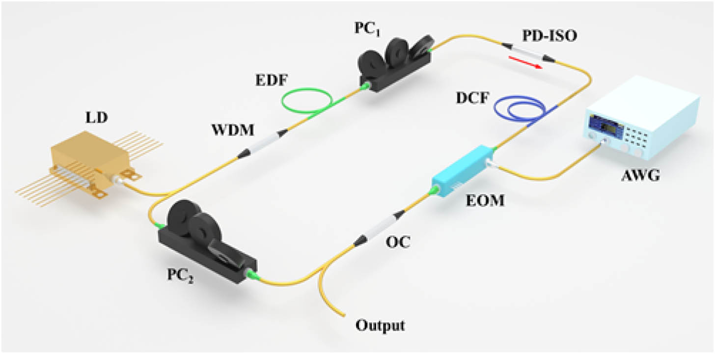
Fig. 1. Laser setup. LD, laser diode; WDM, wavelength division multiplexer; EDF, erbium-doped fiber; DCF, dispersion compensated fiber; PC, polarization controller; PD-ISO, polarization dependent isolator; OC, optical coupler; AWG, arbitrary waveform generator; EOM, electro-optic modulator.

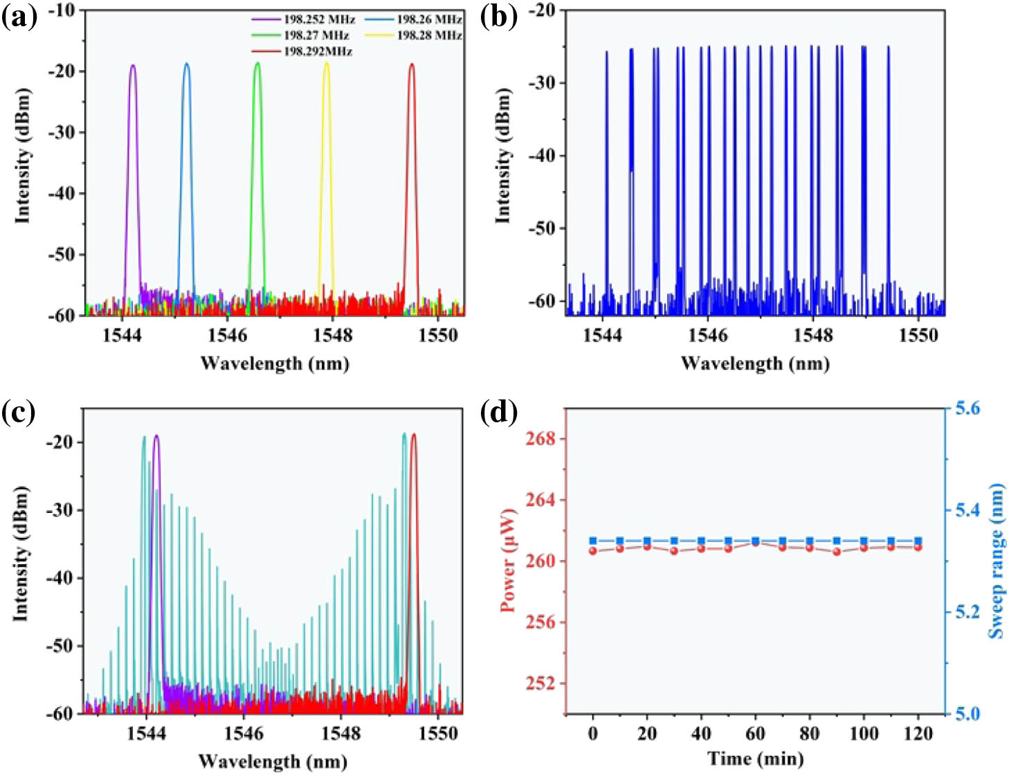
Fig. 2. (a)–(c) Spectra corresponding to sinusoidal signals with different modulation frequencies (fm) generated from the AWG. (a) The fm is 192.252 MHz, 198.26 MHz, 198.27 MHz, 198.28 MHz, and 198.292 MHz, respectively. (b) The fm is rapidly and linearly swept between 198.252 MHz and 198.292 MHz. (c) The fm is switched between 198.252 MHz and 198.292 MHz. The purple and red curves are the same as in (a). (d) The stability of the laser. The red dots represent the output power, and the blue squares represent the sweep range.

Fig. 3. Experimental results of the fm switching process. (a) The intensity dynamics process measured by a high-speed oscilloscope. (b) The blue curve is the integration of the energy of (a), and the red box corresponding to the fm is 198.292 MHz and 198.252 MHz, respectively. (c) The close-up of the yellow dashed box in (a). (d) The close up of the energy integration curve with RT = 4000, and the red circle represents the peak position.

Fig. 4. Experimental results of the fm at the static and sweep periodic cycles. (a) The real-time pulse evolution measured by a high-speed oscilloscope. (b) The blue curve is the integration of the energy in (a), and the red wireframes correspond to the states of the fm at static, NS, PS, and static, respectively. (c) The close-up of the yellow dashed box in (a). (d) The close-up of the energy integration curve near RT=8330, and the red circles represent the data points.

Fig. 5. Experimental results of the fm at PS and NS cycles. (a) The real-time pulse evolution measured by a high-speed oscilloscope, points 1 and 5 correspond to the fm=198.252  MHz, point 3 corresponds to the fm=192.272  MHz, and points 2 and 4 correspond to the fm=198.146  MHz. (b) The blue curves are the integration of the energy in (a). The red wireframes correspond to the states of the fm at PS and NS, respectively. (c) and (d) The energy integration curves of the upper and lower pulses in (a), respectively.

Fig. 6. (a) Linear variation curves of the fm and central wavelength with RTs. (b) The evolution of the spectral linewidth of the pulse below in Fig. 5(a).

Fig. 7. Variation of the partial longitudinal mode of the laser at a wavelength of 1546.59 nm with RTs.

Fig. 8. Simplified model used in simulation. EDF, erbium-doped fiber; DCF, dispersion-compensated fiber; PC, polarization controller; EOM, electro-optic modulator.

Fig. 9. Simulation results. (a) Simulated spectrum evolution in the switching mode. (b) The evolution of the pulse corresponding to (a), (c) the simulated spectrum evolution in the static-sweeping mode, and (d) the evolution of the pulse corresponding to (c).

Table 1. Parameters Used in Simulation