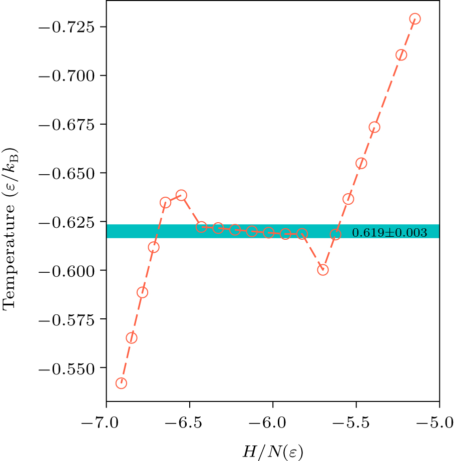
Fig. 1. The gNPT simulation gives the almost constant value of the temperature in the middle of the phase-coexistence energy region as the phase transition temperature T_c = 0.619±0.003ε/k_B for LJ model. Here the temperature as y axis is the calculated interior temperature of the system in the simulations, 1/S′(E), rather than an input parameter.

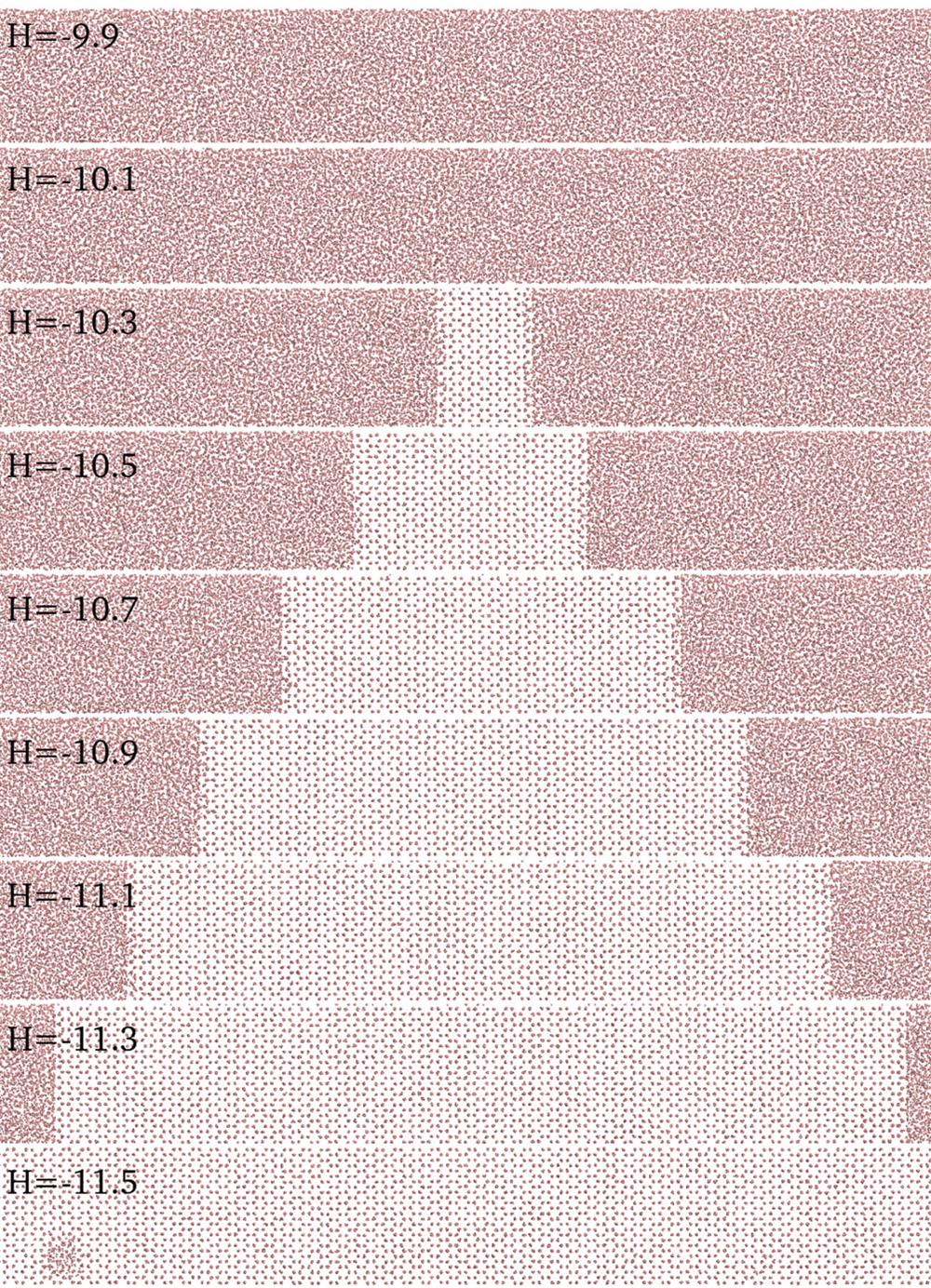
Fig. 2. The stable conformations in the gNPT simulations with distinct enthalpies, from all liquid water, the ice/water coexistence with different fractions of ice and water, to the complete frozen ice I_h.

Fig. 3. The evolution of obtained temperature in gNPTs with distinct parameter. The initial conformation is a coexistent state of ice I_h/water. Only the first 5 ns simulation trajectories are plotted.

Fig. 4. The temperatures obtained in the gNPT simulations. Cyan region refers to 274.6 ± 1 K, the melting point of the mW water model proposed in previous study.^[7]T_c = 275.1 ± 0.3 K is the average of six simulations located in the phase-coexistence region.

Fig. 5. The gNPT method determined the phase transition temperature of the TIP4P-2005 water model. Cyan region refers to 252 ± 5 K from the free energy calculations, yellow region refers to 249±3 K of the direct coexistence route.^[21]

Fig. 6. The gNPT method determines the phase transition temperature for the TIP4P-ICE water model. The melting point (272.2 K) proposed in previous work^[30] is plotted as the dash line.

Fig. 7. Finite-size effect in the gNPT method determines the phase transition temperature. Data from Fig. 4 is shown in black, the other data is extracted from the simulations with 44800, 5971, and 2030 water molecules, respectively.

Table 1. The coexistence temperature of the mW, TIP4P/2005, TIP4P/ice water and LJ models as obtained from different methods (free energy calculations, Hamiltonian Gibbs–Duhem integration, direct coexistence technique, and the current GCE (gNPT) approach).