Abstract
All-optical magnetization switching with features of low-power consumption and high writing speed is a promising road map to satisfy the demand for volume data storage. To promote denser and faster magnetic recording technologies, herein, all-optical helicity-dependent switching (AO-HDS) in multi-layer magnetic recording is proposed based on the chromatic aberration of an optical lens (Thorlabs’s N-BK7 plano-convex uncoated lens). The power of the incident beams and the thickness of the multi-layer magnetic recording film are designed carefully. Besides, the uniformity of this multi-layer magnetic recording is optimized. At last, a prototype system of information multiplexing based on this multi-layer magnetic recording technology is constructed as well. Flexible and controllable magnetization reversals in different layers are also demonstrated by tuning the wavelength and helicity of working beams. We believe that such a prototype system can pave the way for increasing the storage density in an effective and low-cost mode.As conventional two-dimensional (2D) magnetic storage technologies, hard-disk drives have existed for more than half a century and almost reached their performance envelope[1]. Researchers have made enormous attempts at new approaches to promoting denser and faster magnetic recording technologies for a long time[2–4]. All-optical helicity-dependent switching (AO-HDS), where the magnetization can be reversed precisely, is driven by a series of ultrashort optical pulses with left- or right-handed circular polarization, offering a new pathway to satisfy the demand for high-density data storage with low-cost energy and high writing speed, and has attracted considerable attention due to its potential applications[5–8]. The mechanisms of AO-HDS originate from the inverse Faraday effect (IFE) and thermal effect[8–11]. In fact, this process depends largely on the distribution of the optical electric field[1,12–14]. Consequently, tailoring the optical electric field distribution is an effective and simple way to achieve multi-layer magnetic storage.
Based on the aforesaid concept, many new strategies on multi-layer magnetic storage have been provided, e.g., a optical configuration[15–17], a plane wave spectrum method[18–20], and an inverse calculation method with dipole antenna theory[21–23]. However, those three strategies suffer from the complexity of aligning these double optical paths, poor efficiency of the wave spectrum method, and high costs of components employed in the inverse calculation method. These prototype systems face serious practical limitations. Recently, the AO-HDS in a Co/Pt system is surveyed, and the threshold of AO-HDS for the ferromagnet is [24]. When the laser fluence is smaller than the threshold, no switching is performed, and only a demagnetization and slower re-magnetization process exist. However, with the increase of laser energy, AO-HDS is observed. In further increasing the laser energy, thermal demagnetization appears, as the magnetization is heated up to a high temperature, where the ferromagnet cannot cool down, and the resulting value of magnetization will be zero. Hence, when the laser fluence is selected at a proper value, the IFE can determine the switching of the magnetization. To promote denser and faster magnetic recording technologies, based on the chromatic aberration of an optical lens, in this paper, we use a computer to simulate the chromatic aberration of the optical system and demonstrate the possibility of multi-layer magnetic recording by using a tunable laser. The power of the incident beams and the thickness of the multi-layer magnetic recording film are designed carefully, and the magnetic system is heated to just below the Curie point by the femtosecond laser. Besides, a prototype system of information multiplexing is constructed as well, according to this multi-layer magnetic recording technology.
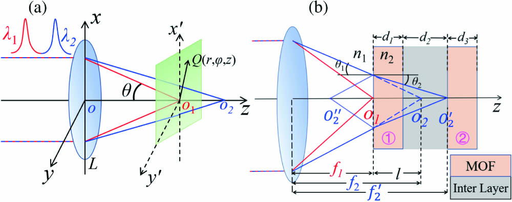
As shown in Fig. 1, two beams with wavelengths and from a dual-wavelength laser[25,26], as an example, are first collected by a Thorlabs objective lens (N-BK7 plano-convex uncoated lens[27]) and then focused towards the interface at and , respectively. The focal length of a plano-convex lens can be calculated as follows: , where is the radius of curvature for the convex surface of the plano-convex lens, and is the refractive index of the lens[27,28]. According to the tutorial of a Thorlabs N-BK7 plano-convex uncoated lens, the refractive index of the objective lens is changed under different wavelengths, as the blue line shows in Fig. 2. As a result, the focal length is altered, which is presented in the pink line (see Fig. 2). In Fig. 2, the radius of curvature of the plano-convex lens selected is .
Sign up for Chinese Optics Letters TOC. Get the latest issue of Chinese Optics Letters delivered right to you!Sign up now

Figure 1.(a) Optical system of layered-resolved all-optical toggling of magnetization. (b) Diagram showing incident beams focused by an objective lens into a two-layer MOF. , objective lens; MOF, magnetic-optic film.
Figure 2.Refractive index and focal length of an N-BK7 plano-convex uncoated lens as a function of the wavelength .
In Fig. 2, the focal length of the uncoated lens can be modeled as an inhomogeneous dependence given by the following expression:
As for two illuminating beams with wavelengths and , their focal lengths are and , respectively. Thereby, when these two beams illuminate the same plano-convex lens, they will be focused at different depths. Consequently, the optical electric field distribution in the image space can be tailored.
According to the vectorial Debye theory, the electric field of these two beams at their focal points can be calculated precisely[28–30]. As the inset shows in Fig. 1(a), in the reference frame for a left-handed circularly polarized incident beam, the field at the image space point can be expressed as where
Here, is the convergence semi-angle of the lens, and , where is the maximum radius of the lens, and we set . is the wave number, is the Bessel function of the first kind, and is a constant, which is determined by the wavelength of the incident beam, the focal length of the lens, and electric field of the incident beam. As the most extensive application of laser technology, Laguerre–Gaussian (LG) beams are widely applied in modern scientific research. The fundamental mode of an LG beam is taken as an example in our simulation. Since most objective lenses obey the sine condition, the constant can be described as the following formula[31]:
In Eq. (4), is another constant representing the amplitude of the incident beam, and is selected in the next simulation. Following the foregoing analysis, the intensity distribution of the focused beam in the focal region can be obtained. According to the IFE, the induced magnetic field in the magnetic-optic film (MOF) can be expressed as where and are the magneto-optical susceptibility of the MOF and the conjugate of the electric field , respectively. In our simulation, the MOF can be GdFeCo[8] or Co/Pt[24], and their switching of magnetization is determined by the helicity of the laser pulse, when the laser fluence is selected at a proper value. Figure 3 presents the intensity distribution and the induced magnetization in the focal region, and the polarization and wavelength of the incident beam are left circular polarization and 780 nm, respectively. Figures 3(a) and 3(c) show the three components of the electric energy () and total electric energy () in the plane and the plane, respectively. Figures 3(b) and 3(d) show the three components of the induced magnetization () and total magnetization () in the plane and the plane, respectively. In Fig. 3, these intensities and the induced magnetization are normalized to the maximum value of the total electric energy and the maximum value of , respectively. From the analysis of Eq. (2), in Figs. 3(a) and 3(b), we can see that the polarization of the focus is left circularly polarized. Thereby, a magnetic field with a positive direction along the axis is induced by IFE [Fig. 3(d3)]. In Fig. 3(d4), it can be found that an optical needle with about in depth and in width is obtained in the focal region. According to Eq. (5), we can find that the distribution of the induced magnetization is relative to the intensity distribution of the focused optical laser[16,17]. Figures 3(a4), 3(b4), 3(c4), and 3(d4) conform to the assumption. Comparing with Figs. 3(c4) and 3(d4), we can see that there is an overlap between the distribution of electric energy and the induced magnetization. Therefore, tailoring the optical electric field distribution is an effective and simple way to achieve multi-layer magnetic storage.
Figure 3.Intensity distributions in the (a) plane and (c) plane, respectively. Induced magnetization in the (b) plane and (d) plane, respectively. The incident beam is left circularly polarized with wavelength . The intensity and the magnetization are normalized to the maximum value of the intensity and magnetization, respectively.
Figure 4.Total intensity distributions on the plane of two focused beams with wavelength (a) and (b) . (c) Cross-section total intensity distribution on the plane.
As revealed before, focusing optical beams with different wavelengths will generate different focal points. Figure 4 shows the total electric energy distributions of two focused beams with different wavelengths on the plane, and the incident beams are left circularly polarized with wavelengths and , respectively. As we have analyzed before, the distribution of the induced magnetization is in accordance with the intensity distribution of the focused optical pulse, and Fig. 4 presents the distribution of the focused optical pulse only. In Fig. 4(a), these two total electric energies are normalized to the maximum value between 780 nm and 800 nm, and we can find that an offset with a value of about 0.01 mm exists between these two foci. Figure 4(b) shows the cross-section total intensity distribution of these two focused beams on the plane, and these two focal points almost have the same energy distributions. Hence, a two-layer magnetic recording can be achieved easily if a two-layer MOF with an interlayer is located after the objective lens, where the two MOF layers are positioned at the two focal planes, respectively.
However, if the two-layer MOF is located at the two focal planes, as shown in Fig. 1(b), where the first layer of the MOF is located at the focal plane , the real focal plane of wavelength will shift a distance to point , due to the mismatch of the refractive indices across the interface[32–34], and this distance is called focal shift[33]. Therefore, the thickness of the interlayer should be designed seriously. Based on the vectorial Debye theory again, the transmitted electric field in this optical system with an interlayer interface could be expressed as[32,33]where
Here, , , and are the cylindrical coordinates of an observation point near the plane, , and , where is the refractive index of the corresponding layer. In Eq. (7), and are the amplitude transmission coefficients of the parallel polarization state and the perpendicular polarization state, and they can be calculated by the Fresnel equation as follows[35]:
In Eq. (7), is a well-known aberration function[33], acquired by the mismatch of the refractive indices of these different layers, and it can be written as where is the probe depth, and the incident angle and the refraction angle are connected through Snell’s law, as shown in Fig. 1(b).
Besides, the wavelength of will also be reflected to across the interface, and the reflected electric field in this optical system can be calculated as follows[35]:
Figure 5 shows the transmission coefficients and reflection coefficients under different , and we can find that most of the energy of the incident beam passes through the interface. Therefore, the reflection on the interface is neglected in this paper.
Figure 5.Transmission coefficients and reflection coefficients under different .
Figure 6 shows the intensity distribution of these two incident beams with wavelengths and in the whole spatial range. The probe depth can be seen in Fig. 6. To simplify the calculation process, we assume that the interlayer has the same refraction as the MOF and the refractive index [8]. Figures 6(a1) and 6(b1) show the electric field intensity distribution and the cross-section total intensity distribution in the focal region. Compared with Fig. 4, we can find that in Fig. 6 the focal shift of is about 0.01 mm, and the full width at half-maximum (FWHM) of the focal point is stretched simultaneously. Due to the mismatch of the refractive indices of these different layers, some energy is reflected, resulting in about a 58% decrease of the focal energy.
Figure 6.Total intensity distribution of the focal fields with different wavelengths in the whole spatial range. (a1), (b1) Amplitude constant . (a2), (b2) Amplitude constant .
In the aspect of three-dimensional (3D) magnetic-optic recording, the uniformity of the focal field amplitude has been applied to evaluate the performance of multi-layer magnetic recording, and the uniformity is routinely defined as , where is the maximum difference among these focal points in the normalized total intensity distribution[16]. To increase the uniformity of these two foci, the amplitude of the second incident beam is increased by tuning the constant to 1.35. As shown in Figs. 6(a2) and 6(b2), the uniformities of these two foci are evaluated as almost 100%, and such a high uniformity can offer an excellent tolerance multi-layer magnetic recording. On the other hand, by controlling the amplitude of the corresponding incident beams, magnetization reversal in different layers, where these MOFs have different coercivity, can also be realized[7–9].
Next, we expand the two-layer magnetic recording to three-layer magnetic recording as shown in Fig. 7, where three incident beams with wavelengths , , and are focused by the same objective lens. According to Eq. (1), the focal length of the third incident beam is . The intensity distributions of these three focal points are shown in Fig. 7, in which the amplitude constant of the second and third incident beams is the same, equaling 1.35. We can find that these three focal points have good uniformity [see Fig. 7(b)]. The FWHMs of these three focal points are about , , and , respectively.
Figure 7.(a) Total intensity distribution of the focal fields with different wavelengths in the whole spatial range. (b) Cross-section total intensity distribution on the plane.
The thickness of the interlayer is calculated as well. As shown in Fig. 1(b), the thickness of the interlayer satisfies , where is the thickness of the first-layer MOF, and is the real focal length of . It is easy to obtain that the thickness of the second interlay , where is the real focal length of . Figure 8 presents the chromatic aberration of the focal lengths under different probe depths . In Fig. 8, we define as the chromatic aberration of the focal length, and , . In Fig. 8, is a monotonically increasing function of , while is a constant with . Due to the foregoing assumption, we propose that the interlayer has the same refractive index as the MOF. In Fig. 7, it can be found that the thicknesses of the first and second interlayers should be larger than the FWHM of the second and third focal points to reduce the interactive influences among different intensity distributions caused by these different incident beams. Therefore, the thicknesses of these two MOFs should be less than and , respectively. In Fig. 8, we can see that when , is about . Consequently, if , the thicknesses of the first and second interlayers are about and , respectively.
Figure 8.Chromatic aberration of the focal lengths under different probe depths .
At last, we also construct a multi-layer magnetic recording system by using a tunable laser, as shown in Fig. 9. As a conceptual illustration, this prototype system consists of an -layer MOF with wavelengths impinging into the MOF, respectively. The different states of the MOF in different layers can be obtained by tuning the wavelengths of the incident beams by a tunable filter[36,37]. Intriguingly, this prototype system can also induce MOF with in-plane states by modulating the polarization of the incident beam[38,39]. As shown in Fig. 9, the red wavelength induces the spin in the first-layer MOF with the “right” state, the blue wavelength induces the spin in the second layer MOF with the “left” state, and the green wavelength induces the spin in the -layer MOF with the in-plane state. In Fig. 9, the polarization of and is left- and right-handed circularly polarized, respectively. As shown in Fig. 10, when the polarization of the induced beam is right-handed circularly polarized light, the induced magnetic fields is along the direction [Fig. 10(b3)][8,30,40], while the intensity distribution in the focal region is the same as the left-handed circularly polarized light [Fig. 10(a)]. The polarization of is hybrid, which can be generated by tailoring the amplitude, phase, and polarization[39], and an oriented in-plane magnetization is induced, resulting in the spin in layer three with the in-plane state.
Figure 9.Scheme of information multiplexing by the multi-layer magnetic recording system. The incident beams are with different wavelengths and polarizations. , left-handed circular polarization; , right-handed circular polarization; , hybrid polarization.
Figure 10.(a) Intensity distributions and (b) induced magnetization in the plane. The incident beam is right circular polarization. The intensity and the magnetization are normalized to the maximum value of the intensity and magnetization, respectively.
In this case, this system shows its potential in multi-layer magnetic recording. In practice, if the polarization, phase, and amplitude of the input beam are further optimized, more states of MOF can be realized. Therefore, this system has great potential applications in information multiplexing. We should also point out that the readout process is another key process in AO-HDS. To readout the data record in different layers of MOF, the magneto-optical Kerr effect, combining with the cross sections extracted from background-corrected magneto-optical images can be applied[1]. Last, but not least, the storage densities can also be promoted by selecting proper incident beams, for example, azimuthally polarized vortex beams[41–43], where the magnetic bits recorded can be reduced to nearly 30%, enabling multi-layer magnetic recording of nanoscale domains. Besides, an oil immersion objective lens with a larger NA can also be applied to further reduce the size of the focal point[44], and the storage densities can be enhanced more.
In summary, according to the chromatic aberration of an optical lens, we investigate the chromatic aberration of the focal lengths of different wavelengths, and a strategy to achieve multi-layer magnetic recording through a tunable laser is proposed in this paper. By tuning the wavelength and helicity of the working beams, the choice of layer of the MOF dictates what is used to record. The thickness of the multi-layers magnetic recording film is designed carefully as well. In addition, the uniformity of this multi-layer magnetic recording is surveyed and optimized. Lastly, the potential for volume data storage of this strategy is explored, and a prototype system of information multiplexing is constructed according to this multi-layer magnetic recording technology. We believe that such a prototype system can present an effective and low-cost step towards high-density storage.
References
[1] D. O. Ignatyeva, C. S. Davies, D. A. Sylgacheva, A. Tsukamoto, H. Yoshikawa, P. O. Kapralov, A. Kirilyuk, V. I. Belotelov, A. V. Kimel. Nat. Commun., 10, 4786(2019).
[2] Y. Wang, D. Zhu, Y. Yang, K. Lee, R. Mishra, G. Go, S. Oh, D. Kim, K. Cai, E. Liu, S. D. Pollard, S. Shi, J. Lee, K. Teo, Y. Wu, K. Lee, H. Yang. Science, 366, 1125(2019).
[3] A. V. Kimel, M. Li. Nat. Rev. Mater., 4, 189(2019).
[4] X. Li, Y. Cao, M. Gu. Opt. Lett., 36, 2510(2011).
[5] F. Siegrist, J. A. Gessner, M. Ossiander, C. Denker, Y. Chang, M. C. Schröder, A. Guggenmos, Y. Cui, J. Walowski, U. Martens, J. K. Dewhurst, U. Kleineberg, M. Münzenberg, S. Sharma, M. Schultze. Nature, 571, 240(2019).
[6] A. Stupakiewicz, K. Szerenos, M. D. Davydova, K. A. Zvezdin, A. K. Zvezdin, A. Kirilyuk, A. V. Kimel. Nat. Commun., 10, 612(2019).
[7] Y. Xu, M. Deb, G. Malinowski, M. Hehn, W. Zhao, S. Mangin. Adv. Mater., 29, 1703474(2017).
[8] C. D. Stanciu, F. Hansteen, A. V. Kimel, A. Kirilyuk, A. Tsukamoto, A. Itoh, T. Rasing. Phys. Rev. Lett., 99, 047601(2007).
[9] A. V. Kimel, A. Kirilyuk, P. A. Usachev, R. V. Pisarev, A. M. Balbashov, T. Rasing. Nature, 435, 655(2005).
[10] K. Vahaplar, A. M. Kalashnikova, A. V. Kimel, D. Hinzke, U. Nowak, R. Chantrell, A. Tsukamoto, A. Itoh, A. Kirilyuk, T. Rasing. Phys. Rev. Lett., 103, 117201(2009).
[11] G. Choi, A. Schleife, D. Cahill. Nat. Commun., 8, 15085(2019).
[12] Y. Xu, M. Hehn, W. Zhao, X. Lin, G. Malinowski, S. Mangin. Phys. Rev. B, 100, 064424(2019).
[13] G. Kichin, M. Hehn, J. Gorchon, G. Malinowski, J. Hohlfeld, S. Mangin. Phys. Rev. Appl., 12, 024019(2019).
[14] X. Lin, Y. Huang, Y. Li, J. Liu, J. Liu, R. Kang, X. Tan. Chin. Opt. Lett., 16, 032101(2018).
[15] Z. Nie, H. Lin, X. Liu, A. Zhai, Y. Tian, W. Wang, D. Li, W. Ding, X. Zhang, Y. Song, B. Jia. Light: Sci. Appl., 6, e17032(2017).
[16] W. Yan, Z. Nie, X. Zhang, Y. Wang, Y. Song. Appl. Opt., 56, 1940(2017).
[17] X. Zhang, Y. Xu, M. Lian, F. Zhang, Y. Du, A. Wang, H. Ming, W. Zhao. J. Opt., 22, 015603(2020).
[18] M. Leutenegger, R. Rao, R. Leitgeb, T. Lasser. Opt. Express, 14, 11277(2006).
[19] C. Hao, Z. Nie, H. Ye, H. Li, Y. Luo, R. Feng, X. Yu, F. Wen, Y. Zhang, C. Yu, J. Teng, B. Luk’yanchuk, C. Qiu. Sci. Adv., 3, e1701398(2017).
[20] J. Guan, N. Liu, C. Chen, X. Huang, J. Tan, J. Lin, P. Jin. Opt. Express, 26, 24075(2018).
[21] G. Rui, Y. Li, S. Zhou, Y. Wang, B. Gu, Y. Cui, Q. Zhan. Photon. Res., 7, 69(2019).
[22] S. Wang, J. Luo, Z. Zhu, Y. Cao, H. Wang, C. Xie, X. Li. Opt. Lett., 43, 5551(2018).
[23] J. Luo, H. Zhang, S. Wang, L. Shi, Z. Zhu, B. Gu, X. Wang, X. Li. Opt. Lett., 44, 727(2019).
[24] X. Zhang, Y. Xu, M. Lian, F. Zhang, Y. Du, X. Lin, A. Wang, H. Ming, W. Zhao. OSA Continuum, 3, 649(2020).
[25] X. Rong, S. Luo, W. Li, S. Jiang, X. Yan, X. Guan, Z. Zhou, B. Xu, N. Chen, D. Wang, H. Xu, Z. Cai. Chin. Opt. Lett., 16, 020016(2018).
[26] Y. Liu, Q. Sheng, K. Zhong, W. Shi, X. Ding, H. Qiao, K. Liu, H. Ma, R. Li, D. Xu, J. Yao. Opt. Express, 27, 27797(2019).
[27] .
[28] B. Richards, E. Wolf. Proc. R. Soc. Lond Ser. A Math. Phys. Sci., 253, 358(1959).
[29] L. Guo, Z. Tang, C. Liang, Z. Tan. Chin. Opt. Lett., 8, 520(2010).
[30] Y. Zhang, J. Bai. Phys. Lett. A, 372, 6294(2008).
[31] B. Chen, J. Pu. Appl. Opt., 48, 1288(2009).
[32] P. Török, P. Varga, Z. Laczik, G. R. Booker. J. Opt. Soc. Am. A, 12, 325(1995).
[33] Z. Zhang, J. Pu, X. Wang. Opt. Commun., 281, 3421(2008).
[34] K. Hu, Z. Chen, J. Pu. Opt. Lett., 37, 3303(2012).
[35] M. Born, E. Wolf. Principles of Optics(1999).
[36] B. Sun, A. Wang, L. Xu, C. Gu, Y. Zhou, Z. Lin, H. Ming, Q. Zhan. Opt. Lett., 38, 667(2013).
[37] H. Ahmad, Z. C. Tiu, S. I. Ooi. Chin. Opt. Lett., 16, 020009(2018).
[38] J. Chen, C. Wan, L. Kong, Q. Zhan. Opt. Express, 25, 8966(2017).
[39] X. Zhang, G. Rui, Y. Xu, F. Zhang, Y. Du, M. Lian, A. Wang, H. Ming, W. Zhao. Opt. Express, 28, 2572(2020).
[40] G. M. Choi, A. Schleife, D. G. Cahill. Nat. Commun., 8, 15085(2017).
[41] S. Wang, X. Li, J. Zhou, M. Gu. Opt. Lett., 39, 5022(2014).
[42] S. Wang, C. Wei, Y. Feng, Y. Cao, H. Wang, W. Cheng, C. Xie, A. Tsukamoto, A. Kirilyuk, T. Rasing, A. V. Kimel, X. Li. Appl. Phys. Lett., 113, 171108(2018).
[43] X. Zhang, G. Rui, Y. Xu, F. Zhang, Y. Du, X. Lin, A. Wang, W. Zhao. Opt. Lett., 45, 2395(2020).
[44] K. Shi, P. Li, S. Yin, Z. Liu. Opt. Express, 12, 2096(2004).