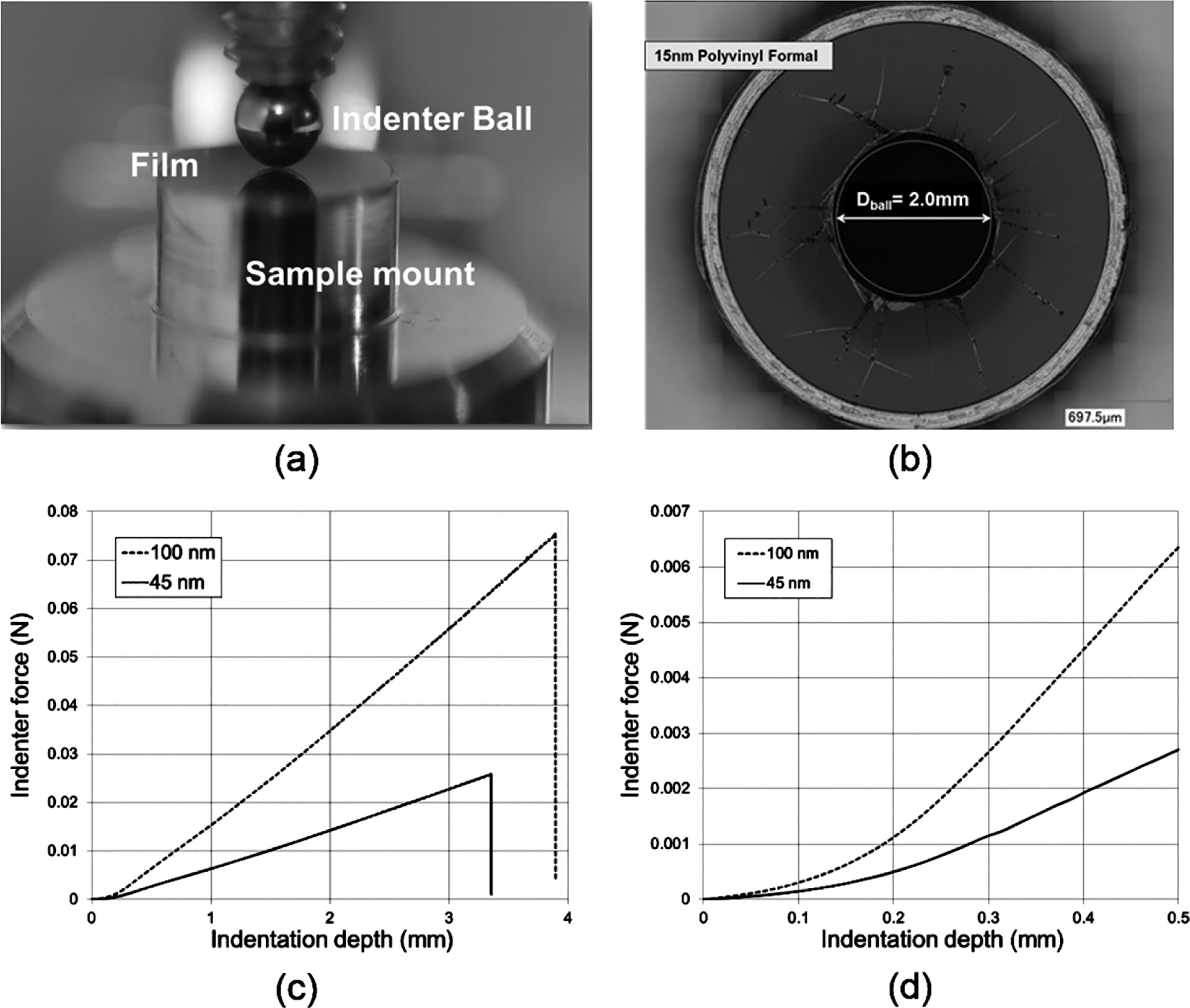
Fig. 1. (a) Indentation test setup consisting of the film mounted onto a sample holder and the indenter ball on a threaded rod, (b) composite photomicrograph of a typical 15 nm polyvinyl formal film following indentation testing to failure. Note the presence of both circumferential and tangential folds suggesting radial and hoop stress induced deformation during loading. The presence and size of the circumferential rupture indicates the predominance of the radial stress state along the contact radius of the indenter, (c) typical curves for ball indenter test showing failure point. The early curve (d) has an almost cubic shape, while the larger indentation depths show an almost linear response.

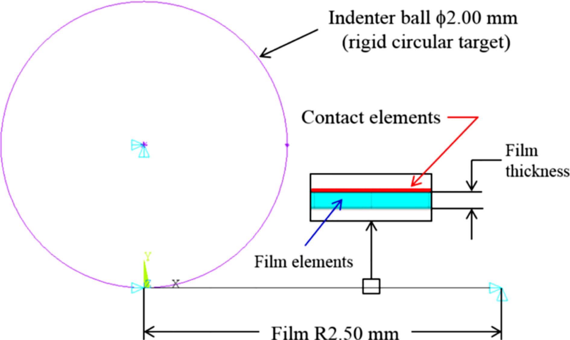
Fig. 2. Axisymmetric finite element model for indentation test, general dimensions of film and indenter ball.

Fig. 3. Typical experimentally determined material respose during an indentation test. The present data was collected for a 100 nm thick polyvinyl formal membrane. Characterized regions of the film material for indentation test.

Fig. 4. Comparison of values derived from a closed-form approximation and experimental indentation data within the elastic portion of the film response. The closed-form approximations, from Ref. [13], were used to estimate a Young’s modulus from the indentation data. The resulting modulus was utilized by the elastic model described in Section 2.3.1 of the text. As shown, even within the elastic portion of the curve, there is poor agreement between the computed and the experimental data (solid line).

Fig. 5. Comparison of experimental and the simulated load/displacement response using optimized elastic parameters ($E$). The optimization algorithm was used to extract elastic parameters ($E=3.28~\text{GPa}$, $\unicode[STIX]{x1D700}_{0}=0.0018$) from the indentation data for a 100 nm thick film. Using these values, modeled and experimental data are in excellent agreement throughout the elastic portion of curve.

Fig. 6. (a) Contour plot for the error metric surface generated from indentation simulation shown in Figure 5. A valley of linear combinations of pre-strain and modulus that all come close to satisfying the equation can be seen. (b) Force versus indentation depth (top) and fit values for different indentation depths (bottom). The fit uses all data points from zero to the given depth. The error of the fit stays low until the behavior transitions from elastic to plastic, between 170 and $190~\unicode[STIX]{x03BC}\text{m}$ of indentation depth, and in this region, the elastic modulus should be read.

Fig. 7. (a) Typical stress–strain curve for a polymer. These complex curves can be approximated with two plasticity materials models in ANSYS, and utilized in the present work. (b) Bilinear model. The material response consists of an elastic response, characterized by an elastic modulus $(E)$ followed, at a yield point ($\unicode[STIX]{x1D70E}_{y}$), by a simple plastic response characterized by a tangent modulus ($E_{T}$). (c) Multilinear model where the material response is described by a series of stress points ($\unicode[STIX]{x1D70E}_{n}$) and their corresponding strain points ($\unicode[STIX]{x1D700}_{n}$).

Fig. 8. A 1 mm indentation depth was simulated with only elastic modulus $(E)$ and pre-strain ($\unicode[STIX]{x1D700}_{0}$), (open circles) and elastic modulus, pre-strain, yield strength ($\unicode[STIX]{x1D70E}_{y}$) and tangent modulus (TanMod) (open diamonds). The elastic regime extends only about $200~\unicode[STIX]{x03BC}\text{m}$ into the indentation. The bilinear model fits the data well for the depth shown, but deviations can already be seen near 0.8 mm indentation, and the difference increases with larger depth. Mechanical properties used for the simulation are $E=3.28$ GPa, $\unicode[STIX]{x1D700}_{0}=0.0018$, $\unicode[STIX]{x1D70E}_{y}=43.50$ MPa, TanMod $=100$ MPa.

Fig. 9. (a) 2 mm indentation simulation. The multilinear simulation result follows the data very well. (b) Optimized multilinear kinematic hardening material model for a film thickness of 100 nm. The inset shows the yield regime in greater detail. The points marked in diamonds on the plot are the points that were entered into the simulation.