Resolution Evaluation Method and Applications of 3D Microscopic Images

Xiliang Luo; Zhou Zhou; Jiangfeng Huang; Xiangjiang Dong; Gang Zheng; Ling Fu

doi:10.3788/CJL202249.0507205

Journals >Chinese Journal of Lasers >Volume 49 >Issue 5 >Page 0507205 > Article

Chinese Journal of Lasers
Vol. 49, Issue 5, 0507205 (2022)

Resolution Evaluation Method and Applications of 3D Microscopic Images

Xiliang Luo^1、2, Zhou Zhou^1、2, Jiangfeng Huang^1、2, Xiangjiang Dong^1、2, Gang Zheng^3、*, and Ling Fu^1、2

Author Affiliations

¹Britton Chance Center for Biomedical Photonics, Wuhan National Laboratory for Optoelectronics, Huazhong University of Science and Technology, Wuhan, Hubei 430074, China

²MoE Key Laboratory for Biomedical Photonics, School of Engineering Sciences, Huazhong University of Science and Technology, Wuhan, Hubei 430074, China

³School of Electronic Information and Communications, Huazhong University of Science and Technology, Wuhan, Hubei 430074, China

show less

DOI: 10.3788/CJL202249.0507205 Cite this Article Set citation alerts

Xiliang Luo, Zhou Zhou, Jiangfeng Huang, Xiangjiang Dong, Gang Zheng, Ling Fu. Resolution Evaluation Method and Applications of 3D Microscopic Images[J]. Chinese Journal of Lasers, 2022, 49(5): 0507205 Copy Citation Text

show less

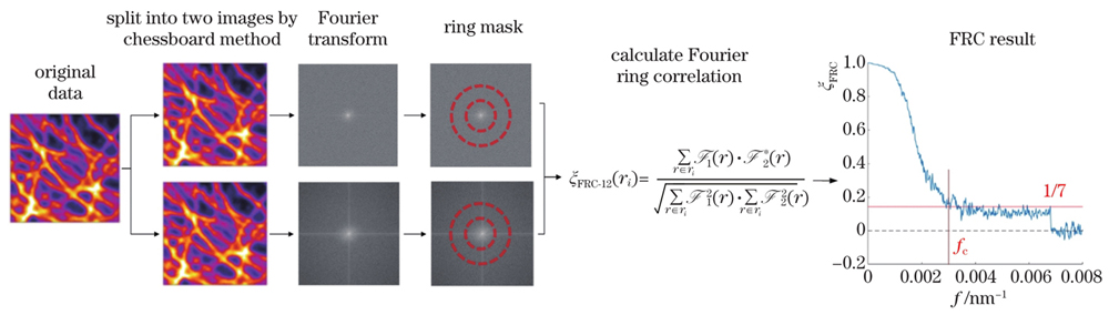
Fig. 1. Flow chart of FRC resolution calculation

Download full size

Working principle diagram of sFSC method’s shell selector. (a) Selector model parameters in spatial diagram；(b) double wedge symmetric selection model; (c) sFSC selector workflow simulation diagram at single frequency shell domain

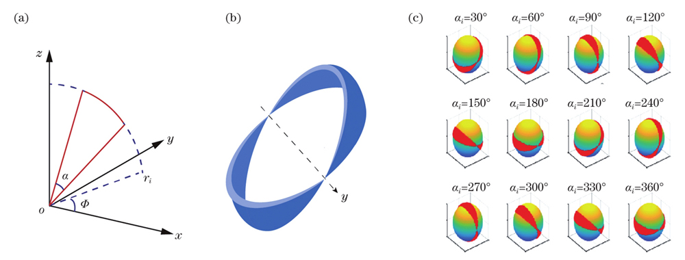
Fig. 2. Working principle diagram of sFSC method’s shell selector. (a) Selector model parameters in spatial diagram；(b) double wedge symmetric selection model; (c) sFSC selector workflow simulation diagram at single frequency shell domain

Download full size

Fig. 3. Resolution evaluation results of fluorescent balls with 0.1 μm diameter. (a) Intensity profile of the fluorescent balls; (b) Gaussian fitting results of intensity profile by FWHM method; (c) angle-dependent resolution curve calculated by sFSC method

Download full size

Fig. 4. Flow chart of image restoration based on sFSC resolution evaluation method

Download full size

Fig. 5. Comparison of resolution and image quality before and after restoration. (a) Resolution curves using sFSC method；(b) image comparison before and after Wiener deconvolution; (c) intensity profile curves of ROI in Fig. 5(b)

Download full size

Fig. 6. Comparison of images reconstructed by Wiener deconvolution under different PSF. (a) Original data; (b) T-PSF; (c) R-PSF1; (d) R-PSF2; (e) O-PSF; (f) sFSC-PSF

Download full size

Fig. 7. Maximum projection images reconstructed by different deconvolution methods on different PSF size

Download full size

Fig. 8. sFSC resolution curves of LW deconvolution with R-PSF and sFSC-PSF input. (a) R-PSF (0.18 μm×0.55 μm)；(b) sFSC-PSF (0.198 μm×0.679 μm)

Download full size

Method	Lateral resolution	Axial resolution
Theoretical	0.292	0.979
FWHM	0.294	1.297
sFSC	0.312	1.648

Table 1. Comparison of resolution results among theoretical calculation, FWHM, and sFSC methods　unit：μm

PSF	Original data	T-PSF	R-PSF1	R-PSF2	O-PSF	sFSC-PSF
Size /(μm×μm)		0.204×0.458	0.18×0.55	0.22×0.60	0.25×0.60	0.198×0.679
Score	4.04	4.94	5.33	5.09	4.82	5.40

Table 2. BIBLE score of the maximum projection images reconstructed by Winner deconvolution on different PSF size

PSF	Original data	T-PSF	R-PSF1	R-PSF2	O-PSF	sFSC-PSF
Size /(μm×μm)		0.204×0.458	0.18×0.55	0.22×0.60	0.25×0.60	0.198×0.679
Lateral resolution /μm	0.1984	0.1737	0.1707	0.1763	0.1814	0.1693
Axial resolution /μm	0.6792	0.4591	0.4610	0.4657	0.5167	0.4538

Table 3. sFSC resolution evaluation results of images reconstructed with Wiener deconvolution on different PSF size

PSF		T-PSF	R-PSF1	R-PSF2	O-PSF	sFSC-PSF
Size /(μm×μm)		0.204×0.458	0.18×0.55	0.22×0.60	0.25×0.60	0.198×0.679
BIBLE score	RL	3.94	4.18	3.78	3.56	4.38
	NNLS	2.85	2.95	2.68	2.50	3.22
	LW	2.86	3.19	2.83	2.66	3.38
	TRIF	2.94	3.36	2.93	2.70	3.51

Table 4. BIBLE score of the maximum projection images reconstructed by different deconvolution methods on different PSF

PSF		T-PSF	R-PSF1	R-PSF2	O-PSF	sFSC-PSF
Size /(μm×μm)		0.204×0.458	0.18×0.55	0.22×0.60	0.25×0.60	0.198×0.679
Lateral resolution /μm	RL	0.1941	0.1820	0.1986	0.2047	0.1725
	NNLS	0.1912	0.1851	0.1969	0.2126	0.1833
	LW	0.1813	0.1705	0.1904	0.2097	0.1824
	TRIF	0.1823	0.1665	0.1916	0.2125	0.1665
Axial resolution /μm	RL	0.6229	0.6178	0.6355	0.6409	0.6160
	NNLS	0.5362	0.5329	0.5283	0.5337	0.5307
	LW	0.5309	0.4999	0.5269	0.5381	0.5013
	TRIF	0.5265	0.5035	0.5208	0.5347	0.5011

Table 5. sFSC resolution evaluation results of images reconstructed by different deconvolution methods on different PSF

Download Citation

Set citation alerts for the article

Tools

Set citation alerts for the article

Save the article for my favorites

Paper Information