


Chao Liu, Jingwei Lü, Wei Liu, Famei Wang, Paul K. Chu, "Overview of refractive index sensors comprising photonic crystal fibers based on the surface plasmon resonance effect [Invited]," Chin. Opt. Lett. 19, 102202 (2021)
- Chinese Optics Letters
- Vol. 19, Issue 10, 102202 (2021)
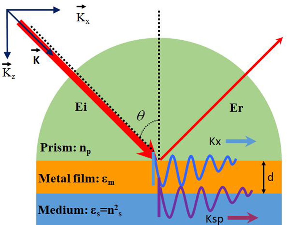
Fig. 1. SPR excitation by prism coupling using the Kretschmann configuration.
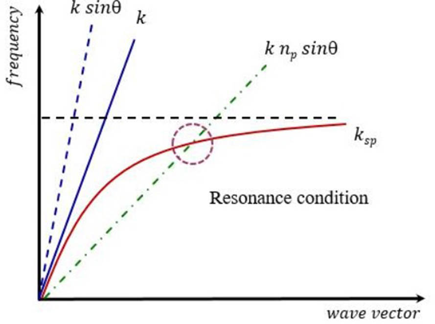
Fig. 2. Dispersion relation of TM incident light coupling with SPP.
Fig. 3. Methodology of SPR measurement: (a) SPR spectra for different RIs and (b) relationship between the wavelength and RI.
Fig. 4. (a) Loss spectra of two PCFs with and without defect. (b) Electronic field distributions of the PCF with defect: insets (c) and (d) show the electronic field distributions of the fundamental core-guided mode and higher-order plasmonic mode at λ = 575 nm; insets (e) and (f) show the energy distribution of the fundamental core-guided mode and fundamental plasmonic mode at λ = 632 nm[57].
Fig. 5. Electronic field distributions of the sensor for different modes: (a) for the core-guided mode, (b) for the plasmonic mode, and (c) for the two modes at resonance point[63].
Fig. 6. (a) Schematic illustration of the side-polished sensor. (b) Dispersion relations and loss spectra of the sensor. (c) Resonant curves for RIs of 1.00–1.20. (d) Resonant curves for RIs of 1.21–1.37[64].
Fig. 7. (a) 2D diagram of the sensor. (b) Three-dimensional (3D) diagram of the sensor. (c) Dispersion relations and loss spectrum of the sensor (red line represents channel 1 for na = 1.35, green line represents channel 2 for na = 1.38). (d) Electric field distributions of the sensor for different wavelengths[68].
Fig. 8. Schematics of the 2D cross section: (a) coated with an Au layer, (b) coated with Au and titanium dioxide layers (TiO2), and (c) coated with the Au-TiO2 grating[74].
Fig. 9. Typical cross-sectional views of various PCF-SPR sensors. (a) Graphene over ITO coated PQF[80]; (b) a Ag core[81]; (c) hexagonal structure consisting of two air hole rings with a central air hole[82]; (d) eccentric core PQF with ITO coating[83]; (e) twin-core PCF with Au coating[84]; (f) analyte filling with Au-Ta2O5 coating[87]; (g) two open-ring channels with Au coating[63]; (h) two parallel D-shaped structures[58].
Fig. 10. (a) General setup for practical sensing; (b) amplitude sensitivity curves of the moisture-monitoring sensor for the x-polarized mode; (c) amplitude sensitivity curves of the moisture-monitoring sensor for the y-polarized mode (d = 0.76 µm, n = 1.330–1.340, dc = 0.3 µm, tg = 40.12 nm, and Λ = 0.8 µm)[114].
Fig. 11. Illustration of the stack-and-draw method for PCF fabrication[125].
Fig. 12. (a) Schematic illustration of HPCVD. (b) Si tubes in a PCF (scale bar: 1 mm). (c) Image of Au nanoparticles array within a 1.6 µm capillary. (d) Image of Au film grown on the inner wall of the Si tube inside PCF (scale bar: 2 µm)[126].
Fig. 13. (a) Schematic of suspended-core fiber front view with Au nanoparticles coating. (b) and (c) SEM images of the inner walls of the suspended-core fiber coated with Au nanoparticles (30 nm diameter spheres): (b) an overview and (c) a zoomed image[127].
Fig. 14. (a) Structure of the SPR sensor and (b) microscopic image of the cross section of the fabricated suspended-core fiber[131].
Fig. 15. SEM images of the cross section of the sputtered fibers[131]: (a) for ∼54 nm Ag film, (b) for ∼66 nm Ag film, and (c) for ∼83 nm Ag film[131].
Fig. 16. (a) Schematic of the plasmonic nanoparticle-functionalized suspended-core fiber and (b) SEM image of the microstructured section of the fiber[132].
Fig. 17. (a) Spliced-fiber pressure-filling technique and (b) optical side views of the splices (left-hand column) and SEM images of the cleaved end-faces (right-hand column); (c) solid-core PCF with all its channels filled with Au, (d) PCF in which only two channels are filled with Au, (e) modified step index fiber with a parallel Au nanowire[134].
Fig. 18. (a) D-shaped model. (b) SEM image of the PCF before polishing. (c) Cross section of the Au-coated D-shaped PCF. (d) Side-polished surface of the D-shaped PCF with a Au coating. (e) Schematic diagram of the real-time online measurement system[121].
Fig. 19. (a) Structure of the sensor. (b) Schematic diagram of the simulated model. (c) Transmitted light microscopic image. (d) Reflected light microscopic image[143].
Fig. 20. (a) End face microscope diagram of PCF. (b) Fusing splice image of MMF-PCF. (c) Schematic diagrams of surface functionalization and immune-sensing process. (d) SEM of Au film on the fiber. (e) Optical properties of the sensor in the immobilization and human IgG[145].
|
Table 1. Refractive Index Ranges of Recently Reported Sensors
|
Table 2. Comparison of the Wavelength Ranges of Recently Reported Sensors
|
Table 3. Comparison of the Characteristics of Selected High Sensitivity of PCF-SPR Sensors Reported Recently
|
Table 4. Comparisons of Plasmonic PCF Sensors


Set citation alerts for the article
Please enter your email address

© Copyright 2018-2021 | Chinese Laser Press. All Rights Reserved 沪ICP备15018463号-20