Normalized point source sensitivity analysis in GSSM prototype

Qichang An; Jingxu Zhang; Fei Yang; Hongchao Zhao

doi:10.3788/COL201715.111202

Abstract

The Giant Steerable Science Mirror (GSSM) is the tertiary mirror of the Thirty Meter Telescope (TMT). To evaluate the performance of GSSM, normalized point source sensitivity (PSSn) is investigated. Calibration and metrology allow the estimation of telescope performance at different zenith angles. PSSn also realizes the prediction of the TMT main mirror assembly optical performance. The relationship between PSSn and slope root mean square (RMS) is analyzed theoretically when evaluating the performance of GSSM. First and foremost, the pointing performance of the GSSM prototype (GSSMP) is specified by PSSn and calibrated by a laser tracker. Then, the tracking performance influence on PSSn is taken into consideration. The jitter of the GSSMP also contributes to the degradation of PSSn, and it is also discussed. Lastly, the interaction between GSSM and the main mirror unit is also revealed by PSSn.

The Thirty Meter Telescope (TMT) is one of the largest telescopes in this world. Its optical system contains a unique tertiary mirror, guiding the light beam to instruments on two science platforms. The Changchun Institute of Optics, Fine Mechanics and Physics, Chinese Academy of Sciences (CIOMP) takes charge of the tertiary mirror that is noted as the Giant Steerable Science Mirror (GSSM). The $3.594 m \times 2.576 m$ flat mirror will point to the instruments on the science platform during telescope tracing. With the goal of understanding and learning, CIOMP will construct a quarter-scaled prototype, realizing the performance of a large plate under a gravity load, high accuracy pointing at a different zenith angle, and minimizing jitter at low speed tracking^[1–3].

To achieve the specification of the GSSM prototype (GSSMP) performance, a suitable index is required. When the index releases enough information, the single index is better than a standard in terms of the form of curve. Normalized point source sensitivity (PSSn) is a well suited index for large telescope performance top-down error budgeting and bottom-up verification^[4,5]. It is first used in the TMT M1 system error allocation and verification. Its perfect multiplicative property refers to overall performance distribution, which is almost equal to the product of the subsystem performance distribution. The misalignment and vibration will result in the degradation of optical performance, for example. Similar to added-on subsystems, the misalignment and vibration are treated as independent error sources. At the same time, root mean square (RMS) of the wave front slope is easily calculated^[6]. Evaluation based on the slope allows for the specification of frequency characteristics. However, RMS is only the second moment of data. In normal conditions, the slope calculation can reduce the influence of the fiducially error by subtracting the nearby data.

The relation between slope RMS and PSSn can be established by analysis. Differences of the mirror figure data will reach the slope data. Slope RMS is accessed by PSSn though power spectral density (PSD). Pointing performance is an important requirement. With the help of the atmosphere structure function, slope RMS and PSSn are related to pointing performance. The tracking jitter is a key performance of the GSSMP. The degradation of GSSMP optical transmission capacity is evaluated by slope RMS and PSSn. The requirement is very demanding, requiring an understanding of the sources of jitter error and improving the performance^[7–9].

Sign up for Chinese Optics Letters TOC. Get the latest issue of Chinese Optics Letters delivered right to you！Sign up now

From the aspect of system engineering, it is always confusing to find an index, considering both the atmosphere and the influence of telescope itself. Point source sensitivity (PSS) is an index to realize in the following: $PSS = \iint {| {OTF}_{atm} (\vec{f}) {OTF}_{tel} (\vec{f}) |}^{2} d \vec{f}$

The optical transfer function (OTF) of atmosphere is ${OTF}_{atm} (\vec{f}) = e^{[- 3.44 {(\frac{λ \vec{f}}{r_{o}})}^{5 / 3}]}$ , where $r_{0}$ is the atmosphere relation length. The OTF of a telescope is ${OTF}_{tel} (\vec{f}) = \iint A (\vec{r}) P (\vec{r}) P (\vec{r} - λ \vec{f}) A (\vec{r} - λ \vec{f}) d \vec{r}$ , where $A (\vec{r})$ is the function of the aperture. $P (\vec{r})$ is the wide pupil function. $λ$ is the wavelength.

Similar to the Strehl ratio, when the PSS is normalized by the OTF of the atmosphere, the normalized index is easy to check and understand.

So, PSSn is computed as $PSS n = \frac{\iint {| {OTF}_{atm} (\vec{f}) {OTF}_{tel} (\vec{f}) |}^{2} d \vec{f}}{{\iint | {OTF}_{atm} (\vec{f}) |}^{2} d \vec{f}} .$ (1)

The OTF of atmosphere is ${OTF}_{atm} (\vec{f}) = e^{[- 3.44 {(\frac{λ \vec{f}}{r_{o}})}^{5 / 3}]}$ , where $r_{0}$ is the atmosphere relation length. The OTF of the telescope is ${OTF}_{tel} (\vec{f}) = \iint A (\vec{r}) P (\vec{r}) P (\vec{r} - λ \vec{f}) A (\vec{r} - λ \vec{f}) d \vec{r}$ . Slope RMS is for the wave front slope. It is related to the prime ripple of the figure under calculation. In order to suppress the fiducially error and highlight the frequency characteristics, slope RMS is employed. Slope RMS is calculated as $Slope {RMS}^{2} = 〈 {| \nabla \cdot Φ |}^{2} 〉,$ (2)where $Φ$ is the wave front under evaluation, and $〈 \cdot 〉$ stands for the averaging over the all of the wave front.

Similar to RMS, slope RMS is hard for composing a large amount of error sources. Subsystems will result in the degradation of the large telescope’s overall performance. What is worse, different frequency components will bring more difficulties to the error budget. It is impossible to allocate or verify errors in such a large system without metric specifying frequency information.

Besides, it is necessary for the systems engineer to understand the relationship between slope RMS and PSSn, so that the slope RMS value can be found equivalent to the PSSn requirement.

Equal to Zernike polynomials, the discrete Fourier series is a completed description of the wave front, specifically, a simpler presentation.

Similar to the Zernike polynomials, the wave front can be expressed by the Fourier series, as is shown in $Φ (m, n) = \sum A_{u v} W_{u v} (m, n),$ (3)where $A_{u v}$ is the coefficient of the fitting, $W_{u v} (m, n)$ is a basic function in an $N \times N$ sampling aperture， and $W_{u v} (m, n) = \frac{1}{N \times N} \exp [\frac{2 π j}{N} (u m + v n)]$ .

To simplify the presentation, the image part of $W_{u v} (m, n)$ is employed for theoretic analysis.

The PSD of the sine-formed wave front $A_{i} \sin (2 π f_{x} x)$ is shown as $PSD (f_{x}) = \frac{{〈 {| A_{i} \sin (2 π f_{x} x) |}^{2} 〉}_{x}}{Δ f_{x}} = \frac{A_{i} Δ f_{x}}{2},$ (4)where $A_{i}$ is the amplitude of the $i_{th}$ sine function, and $f_{x}$ is the spatial frequency. In the spatial frequency domain, the difference is accessible to the product by $f_{x}$ . The relation between PSD and slope RMS is shown in $Slope {RMS}^{2} = {〈 {| \nabla \cdot Φ |}^{2} 〉}_{x} = 2 π^{2} \int_{0}^{\infty} PSD (f_{x}) f_{x}^{2} d f_{x} .$ (5)

On the other hand, PSD is related to PSSn by $1 - PSS n = \int_{0}^{\infty} β (f_{x}) PSD (f_{x}) {(\frac{2 π}{λ})}^{2} d f_{x},$ (6)where $β (f) = {\begin{matrix} μ r_{0}^{2} f^{2} (f < \frac{1}{r_{0}} circle / rad) \\ 2 (f \geq \frac{1}{r_{0}} circle / rad) \end{matrix}$ , and $μ$ is a constant of 2.22.

The weighted slope RMS is a better index for the specification of a large telescope. A single slope RMS requirement for all conditions is the current approach; however, the slope RMS will present more information when more conditions are considered. In both the time and spatial domains, weighted slope RMS is employed.

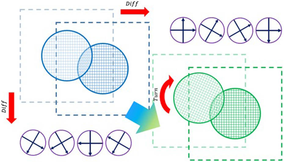
In the spatial domain, the traditional calculation of slope RMS is accessed in relation to the difference in two directions. However, the difference the other directions may also present important information. Setting a coordinate system on the wave front under test, the original one is $(x_{i}, y_{i}, z_{i})$ , and the one after rotation is $(x_{b}, y_{b}, z_{b})$ . The data are turned relatively by $θ$ . After rotation, the difference will be accomplished after interpolation, $[\begin{matrix} x_{b} \\ y_{b} \\ z_{b} \\ 1 \end{matrix}] = [\begin{matrix} \cos θ & \sin θ & 0 & 0 \\ - \sin θ & \cos θ & 0 & 0 \\ 0 & 0 & 1 & 0 \\ 0 & 0 & 0 & 1 \end{matrix}] [\begin{matrix} x_{i} \\ y_{i} \\ z_{i} \\ 1 \end{matrix}] .$ (7)

The wave front is turned $M$ times. It is decided by the calculation cost and characteristics of the figure itself. The procedure of rotation-averaging slope RMS calculation is shown in Fig. 1.

Figure 1.Procedure of rotation-averaging slope RMS calculation.

In the time domain, different zenith angles and targeted instruments are related to a certain probability, $P_{j}$ , $j = 1 \dots N$ . Here, the probability calculation is based on a 30° zenith angle, because the alignment and phasing system (APS) effectively calibrates the telescope to an extent, as well as the diffraction limit, implying that the zenith 30° angle is a reasonable representative average zenith angle.

Hence, the final weighted PSSn is computed as shown in $1 - PSS n = \int_{0}^{\frac{1}{r_{0}}} μ r_{0}^{2} f_{x}^{2} PSD (f_{x}) {(\frac{2 π}{λ})}^{2} d f_{x} + \int_{\frac{1}{r_{0}}}^{\infty} 2 PSD (f_{x}) {(\frac{2 π}{λ})}^{2} d f_{x} \approx \frac{2 μ}{M λ^{2}} \sum_{j = 1}^{N} \sum_{i = 1}^{M} P_{j} \times r_{0 j}^{2} Slope {RMS}_{i, j}^{2},$ (8)where $r_{0 j}$ is the atmosphere relation length at the $j_{th}$ condition. The slope RMS of the GSSM passive support shall satisfy $Slope RMS (ζ) \approx Slope {RMS}_{@ ζ = 0 °} (1 - \frac{\sin ζ}{\sqrt{2}}),$ (9)where $ζ$ is the telescope zenith angle, and $Slope {RMS}_{@ ζ = 0 °}$ is the slope RMS at the zenith angle equaling 0.

The atmosphere relation length at $r_{0} (ζ) = r_{0 @ ζ = 90 °} \cos^{2 / 3} (ζ)$ presents the atmosphere degradation effect as the zenith angle increases. The GSSMP figure at different zenith angles is shown in Fig. 2. The left panel is the case when the zenith angle is 0 and the slope RMS is 0.225 μrad, and the right panel is the case when the zenith angle is 30° and the slope RMS is 0.149 μrad. It meets the specifications of Eq. (7).

Figure 2.GSSMP figure at different zenith angles.

The calculation of the slope RMS is concerned about the spatial sampling grid size. In the left panel of Fig. 3, the simulation is done to profile the relation between the slope RMS and grid size. If the grid size is chosen from 3 to 3.5 mm, the slope RMS is approximately 0.8–0.85 μrad. At the same time, in the right panel, the according PSSn is 0.996 to 0.998.

Figure 3.PSSn and slope RMS versus the GSSMP spatial sampling grid size.

For the pointing performance, according to the definition of full width and half-maximum (FWHM), the FWHM $θ$ and atmosphere structure function $D_{atm} (r)$ are related by $θ = 0.95 \frac{λ}{r_{0}}, D_{atm} (r) = {(\frac{λ}{2 π})}^{2} 6.88 {(\frac{r}{r_{0}})}^{5 / 3} = {(\frac{λ}{2 π})}^{2} 6.88 {(\frac{θ r}{0.95 λ})}^{5 / 3},$ (10)where $λ$ is the wavelength, $r_{0}$ is the atmosphere relation length, and $r$ is the evaluating scale.

According to the definition of slope RMS, the slope RMS of the sine-formed wave front $A_{i} \sin (2 π f_{x} x)$ is shown as $Slope {RMS}^{2} = 〈 {| \nabla \cdot Φ |}^{2} 〉 = 2 π f_{x}^{2} A_{i}^{2} .$ (11)

Setting $f_{o} = \frac{slope RMS}{\sqrt{2} π A}$ as the cutoff frequency of the system, the sine-formed wave front $A_{i} \sin (2 π f_{x} x)$ is supposed to be dominating the wave front aberration. At the same time, the wave front structure function is shown in $D (r) = 2 σ_{ϕ}^{2} {1 - \exp [- {(f_{o} r)}^{2}]},$ (12)noting that $σ_{ϕ}$ is the RMS of the wave front. Setting $σ_{ϕ} = λ / K_{K > 50}$ , $f_{o}$ is the cut off frequency. $r$ is the evaluating scale, and $λ$ is the wavelength. Setting $D_{atm} (r) = D (r)$ , the relationship between the FWHM $θ$ and slope RMS is shown in $Slope RMS = 2 π \frac{λ}{K r_{e}} \sqrt{- \ln [1 - {(\frac{K}{2 \sqrt{2} π})}^{2} 6.88 {(\frac{θ r_{e}}{0.95 λ})}^{5 / 3}]} .$ (13)

$OTF$ due to internal and outside vibration during tracking is in a form of the zero-order Bessel function^[10]. What is more, the energy is introduced to GSSMP, as the settling, slewing, and tracking is processed. OTF under vibration is shown in $OTF (\vec{f}) = B_{0} (D 2 π \vec{f}) .$ (14)

Here, $D$ is the amplitude, $f$ is the frequency, and $B_{0}$ is the zero-order Bessel function.

The multiplied OTF is the product of OTF according to a different component in one piece of frequency, according to the principle of energy. Rewriting Eq. (14), the OTF will be reached by $OTF (\vec{f}) = \prod_{i = 0}^{N_{PSD}} B_{0} (\sqrt{2 Δ ω_{i} {PSD}_{ave, i}} 2 π \vec{f}),$ (15)noting that $Δ ω_{i} = ω_{i + 1} - ω_{i}$ , and ${PSD}_{ave, i} = \frac{PSD (ω_{i}) + PSD (ω_{i + 1})}{2}$

Tracking is the most important and demanding performance. The testing is limited by the minimum velocity command that could be generated by the controller.

Due to the influence of mass, inertia, resonant frequencies, bearings, drives, encoders, and servo bandwidth, the servo system will respond to encoder noise within the loop bandwidth. Noise will contribute to the system jitter. The jitter at 3.6 inch/s speed at the zenith angle of 10° is shown in Fig. 4. The amplitude of Eq. (15) is the modulation transfer function (MTF). By MTF, the influence of the GSSMP optical transmission performance under jitter will be calculated. In Fig. 5, the left panel is the wave front at zenith angle of 10°, and the right panel is the wave front under vibration degrading.

Figure 4.Profile for tracking testing at varied zenith angles.

Figure 5.GSSMP figure under vibration.

In conclusion, subsystems involve degradation to the overall performance of the large telescope. Different frequency components result in more difficulties to the error budget. PSSn and slope RMS are investigated to overcome these problems. Combined with the easy approach of slope RMS and multipliable characteristics, the error of the complicated system is able to be allocated and verified.

References

[1] L. Stepp. Proc. SPIE, 8444, 84441G(2012).

[2] M. K. Cho. Performance prediction of the TMT tertiary mirror, Ritchey–Chrétien design(2007).

[3] G. Z. Angeli, S. Roberts, K. Vogiatzis. Proc. SPIE, 7017, 701704(2008).

[4] B. J. Seo, C. Nissly, G. Angeli, B. Ellerbroek, J. Nelson, N. Sigrist, M. Troy. Proc. SPIE, 7017, 70170T(2008).

[5] G. Z. Angeli, B. J. Seo, C. Nissly, M. Troy. Proc. SPIE, 8127, 812709(2011).

[6] F. Yang, G. Liu, Q. An, X. Zhang. Chin. Opt. Lett., 13, 041201(2015).

[7] D. G. MacMartin, P. M. Thompson, M. M. Colavita, M. J. Sirota. IEEE Trans. Control Syst. Tech., 22, 58(2014).

[8] Y. Bao, X. Yi, Z. Li, Q. Chen, J. Li, X. Fan, X. Zhang. Light Sci. Appl., 4, e300(2015).

[9] S. Poupar, P. Haguenauer, J. Alonso, N. Schuhler, J. P. Henriquez, J. P. Berger. Proc. SPIE, 9145, 91452M(2014).

[10] D. Wulich, N. S. Kopeika. Opt. Eng., 26, 266529(1987).