Fig. 1. Anisotropic-σm hyperbolic metasurface. (a) Schematic view of in-plane negative refraction based on the designed hyperbolic metasurface. The hyperbolic metasurface in the right region is rotated by 90°, comparing with the left one. The black arrows indicate the power flow. (b) Left panel: photograph of the fabricated sample. The sample is composed of arrays of coiling copper wires patterned on dielectric substrates. Right panel: details of a unit cell. Here, a=15.2  mm, b=9  mm, r=2  mm, t=2  mm, w=0.2  mm, and g=0.2  mm. The relative permittivity of the substrate is 3.5+0.001i. The thickness of copper wires is 0.035 mm. The number of coil turns is 14. (c) Numerically-calculated Im(σm) of the metasurface. Blue (red) solid line represents values of Im(σxx) [Im(σyy)]. Black dashed line denotes a value of zero. (d) Iso-frequency contours of the hyperbolic metasurface in the first Brillouin zone. The frequency values are normalized by (c/a)×10−2.

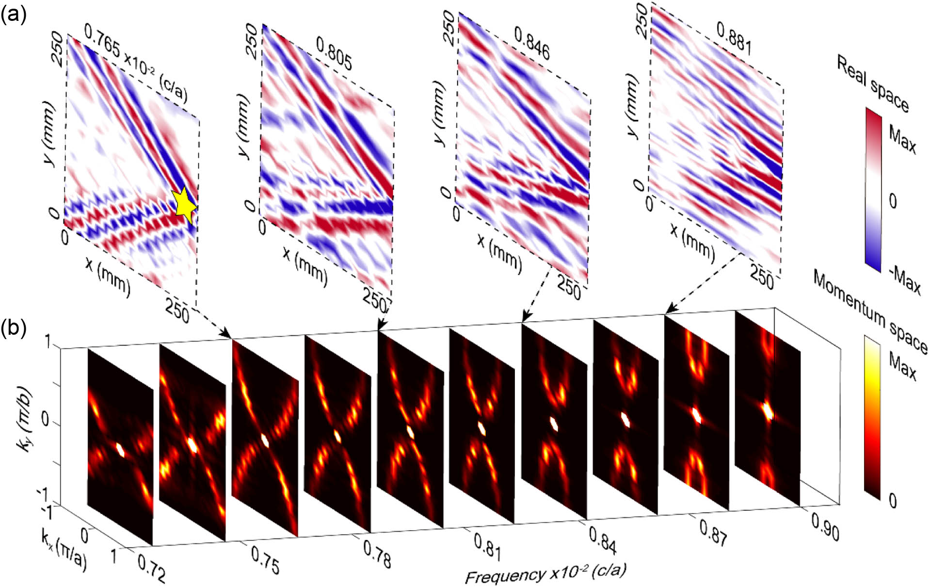
Fig. 2. Measured magnetic field distributions and iso-frequency contours. (a) Measured magnetic patterns of Hz field in the real space on the xy plane 3 mm over the hyperbolic metasurface at 0.765×10−2(c/a), 0.805×10−2(c/a), 0.846×10−2(c/a), and 0.881×10−2(c/a), respectively. The yellow star indicates the source position. The color bar measures the real part of Hz. (b) Iso-frequency contours in the momentum space obtained by applying spatial Fourier transform to the corresponding complex Hz field. The color bar measures energy intensity.

Fig. 3. Achieving an ultra-high squeezing factor in our hyperbolic metasurface. (a) Retrieved squeezing factors of the designer polaritons from simulated and experimental results. An ultra-high squeezing factor of 129 at 0.76×10−2(c/a) is observed. (b) Measured momentum space at 0.76×10−2(c/a). The color bar measures the energy intensity. (c) Measured Hz field on the xy plane 3 mm over the hyperbolic metasurface at 0.76×10−2(c/a). The excitation is marked as a yellow star. The color bar measures the real part of Hz.

Fig. 4. Experimental validation of all-angle in-plane negative refraction of ultra-high-k designer polaritons. (a) Measured Hz field on the xy plane 3 mm above the hyperbolic metasurface at 0.75×10−2(c/a), indicating negative refraction. The vertical black dashed line denotes the interface. The horizontal black dashed lines are normals. The excitation is marked as a yellow star. The yellow arrows represent the directions of the power flow. The color bar measures the real part of Hz. (b) Measured momentum space of the hyperbolic designer polaritons in the left and right regions at 0.75×10−2(c/a), respectively. The green arrows indicate the directions of group velocities (power flow). The color bar measures energy intensity. (c) Measured Hz field at 0.735×10−2(c/a), 0.765×10−2(c/a), and 0.775×10−2(c/a), respectively.

Fig. 5. Side and top views of magnetic field distributions of eigenmodes, respectively. The color bar measures the amplitude of the magnetic field.

Fig. 6. Influence of different geometry parameters on the magnetic hyperbolic polaritons. (a) Dispersions of the metasurface with different periodicity along the x axis (a′). Other parameters keep constant, i.e., b′=9  mm, n′=14, and t′=2  mm. (b) Dispersions of the metasurface with different periodicity along the y axis (b′). Other parameters keep constant, i.e., a′=15.2  mm, n′=14, and t′=2  mm. (c) Dispersions of the metasurface with different number of turns of coils (n′). Other parameters keep constant, i.e., a′=15.2  mm, b′=9  mm, and t′=2  mm. (d) Dispersions of the metasurface with different thickness (t′). Other parameters keep constant, i.e., a′=15.2  mm, b′=9  mm, and n′=14.

Fig. 7. Analytical and simulated iso-frequency contours. (a) Iso-frequency contours obtained from theoretical analysis. (b) Iso-frequency contours obtained from numerical simulations. The frequency values are normalized by (c/a)×10−2.

Fig. 8. (a) Measured momentum space at 0.765×10−2(c/a). The color bar measures the energy intensity. (b) Measured Hz field on the xy plane 3 mm over the hyperbolic metasurface at 0.765×10−2(c/a). The excitation is marked as a yellow star. Here, the green arrows in (a) and (b) depict the direction of group velocity (energy flow) of the high-k modes. (c) Measured Hz field by flipping the x axis of the field in (b). The green dashed curves depict the wavefronts of the hyperbolic polaritons. The color bar measures the real part of Hz.

Fig. 9. Design of a far-infrared hyperbolic metasurface. (a) Schematic of a far-infrared hyperbolic metasurface consisting of coiling silver wires. Yellow area: coiling silver wires. White dashed line: a unit cell. Here, the brown area represents air in order to make the structure look clear. (b) Details of a unit cell. Here, a=1.9  μm, b=1.16  μm, r=0.2  μm, w=0.1  μm, and g=0.1  μm. Number of coil turns is n=4. The thickness of coiling silver wires is 0.1 μm. (c) Three-dimensional perspective view of the dispersion relations of the far-infrared hyperbolic metasurface in the first Brillouin zone. (d) Iso-frequency contours of the metasurface. The hyperbolic contours range from 5.0 to 6.4 THz. The frequency values are presented in the unit of terahertz.

Fig. 10. Experimental setup. (a) A source, which is a broadband antenna, is directly welded on a coil unit cell at the metasurface edge. Green resin structure is used to sustain the hyperbolic metasurface. (b) A detector is a compact coil antenna with magnetic resonance around 0.806×10−2(c/a). The coil-like detector oriented in the direction, is fixed at a robotic arm of a moving platform and moves on the plane 3 mm above the designed hyperbolic metasurface. The inset represents the details of the detector.

Fig. 11. Scheme view of the fields around the hyperbolic metasurface and the coil antenna as a detector.