
Jie Shi, Yulin Liu, Shengguo Shi, Anding Deng, Hongdao Li. Inversion method of bubble size distribution based on acoustic nonlinear coefficient measurement[J]. Chinese Physics B, 2020, 29(8):
- Chinese Physics B
- Vol. 29, Issue 8, (2020)
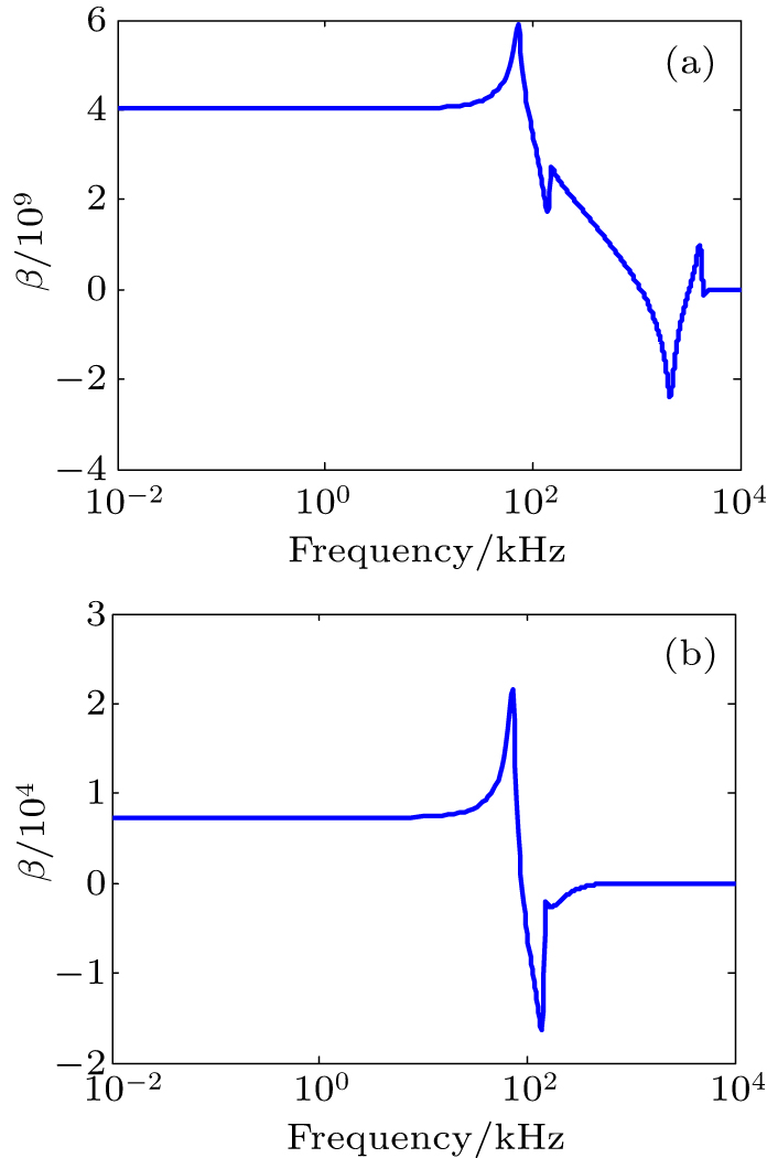
Fig. 1. Nonlinear coefficients under assumed distribution.
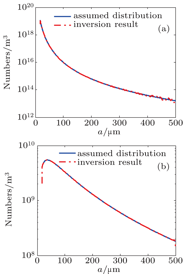
Fig. 2. Inversion results of nonlinear coefficient method.
Fig. 3. Error analysis of inversion results from nonlinear coefficient method: [(a)–(d)] 1%-G, 3%-G, 5%-G, and 10%-G distributions, respectively; [(e)–(h)] 1%-PL, 3%-PL, 5%-PL, and 10%-PL distributions, respectively.
Fig. 4. Error analyses of inversion results of DF inversion method: [(a)–(d)] 1%-G, 3%-G, 5%-G, and 10%-G distributions, respectively; [(e)–(h)] 1%-PL, 3%-PL, 5%-PL, and 10%-PL distributions, respectively.
Fig. 5. Error analyses of inversion results of SH inversion method: [(a)–(d)] 1%-G, 3%-G, 5%-G, and 10%-G distributions, respectively; [(e)–(h)] 1%-PL, 3%-PL, 5%-PL, and 10%-PL distributions, respectively.
Fig. 6. Experimental settings of measuring nonlinear coefficients of bubble medium.
Fig. 7. Experimental system block diagram.
Fig. 8. Nonlinear coefficients measured in experiment.
Fig. 9. Results of bubble size distribution retrieved by NC inversion method.
Fig. 10. Results of bubble size distribution retrieved by SH inversion method.
Fig. 11. Expected inversion effect under experimental conditions.
Fig. 12. Inversion effects of β data in different frequency ranges.
|
Table 1. Comparison of condition number among three inversion methods.
|
Table 2. Comparison of correlation coefficient between inversion and assumed distribution after adding errors under NC inversion.
|
Table 3. Comparison of correlation coefficient between inversion and assumed distribution after adding errors under DF and SH inversion.


Set citation alerts for the article
Please enter your email address

© Copyright 2018-2021 | Chinese Laser Press. All Rights Reserved 沪ICP备15018463号-20