Eco-efficiency is considered to be a measure of coordinated development of economy, resources, environment and ecology, and is therefore an important issue currently. Eco-efficiency can not only provide effective metrics for sustainable development but also comprehensively reflect economic resources and the actual level of coordinated development of environmental-ecological complex systems. Hence, many studies have been done in the academic community on the issue of regional eco-efficiency. Relevant literature focuses on the analysis and evaluation of the concepts and connotations of eco-efficiency, evaluation indicators, measurement methods and models, the relationship between eco-efficiency and economic development factors, the quantitative evaluation of different scale systems, convergence and influencing factors, the timing of eco-efficiency and the characteristics of change and spatial differences. Research areas involve enterprises, industries, regions and countries. At the provincial and industrial levels (Shi, 2006; Wei et al., 2007; Wang and Qu, 2010; Chen, 2014), different definitions of eco-efficiency are given for different application areas and analytical perspectives. Eco-efficiency also employs multiple measurement indicators (Patterson, 1996; Wei and Liao, 2010). The quantitative measurement methods are also different: the ratio method (Duan, 2001; Dahlström and Ekins, 2005; Yacooub and Fresner, 2006; Pan and Ying, 2013), comprehensive index method (e.g. Jollands et al., 2004; Chen, 2008; Wu et al., 2012), material flow analysis (e.g. Chen et al., 2003; Cai et al., 2006; Wang and Shi, 2008; Wu et al., 2009; Zhang et al., 2009; Charmondusit and Keartpakpraek, 2011), ecological footprint method (e.g. Wackernagel and Rees, 1997; Gu, 2005; Wackernagel et al., 2005; Rees and Wackernagel, 2008; Yu, 2009; Zhang, 2011) and data envelopment analysis (e.g. Li and Chen, 2008; Zhang et al., 2008; Deng et al., 2011; Gao et al., 2011; Mahlberg et al., 2011; Oggioni et al., 2011; Sahoo et al., 2011; Wang and Zhu, 2011; Wen and Li, 2011; Chen and Delmas, 2012; Yang et al., 2012; Halkos and Tzeremes, 2013; Pan et al., 2013; Chen et al., 2015) have been widely used. The emerging ecological cost index (Cagno et al., 2012; Vogtländer et al., 2002) and the sociological method (Mickwitz et al., 2006) were also used in recent years. Despite different studies focusing on different themes of eco-efficiency by international organizations, the basic ideas are the same, i.e., from the perspective of input and output for the entire region or individual cities, industrial enterprises, etc. Studies on eco-efficiency indicate that regional eco-efficiency is a composite system that covers all aspects of economy, resources and environment. In addition, the study of eco-efficiency has changed from being just a simple assessment to becoming a driving mechanism abroad. In China, related studies mainly focus on large-scale eco-efficiency evaluation of industries, ecological parks, cities and regions. Hence, this study takes 129 geodesic cities in the Yangtze River Economic Zone (YREZ) as the research unit, measures the eco-efficiency and analyzes the spatial pattern distribution and evolutionary law of eco-efficiency from the spatial dimension.

Over the past 30 years, China has experienced rapid development of reform and opening up, its economic and social development have entered a “new normal”. Whether it can achieve economic growth under the new normal and coordinated development of resources and environment, and get rid of the current “high energy consumption, high pollution and low development dilemma of efficiency and inconsistency to realize ecological priority and green development are important challenges to regional strategic development since the 18th National Congress in 2012. The ecological development path, taking social, economic and resource environment into account, will eventually be the inevitable choice for the future development of China's regions. Although the economy of the Yangtze River Economic Zone (YREZ) has developed rapidly over recent decades, the rationality and ecological protection of development and utilization have not been considered. This has resulted in a decline in the quality of the ecological environment over the whole region because of the intense human activities and long-term development.

If the current course of development and exploitation is not stopped and constrained, it will affect China's overall eco-environment. The State Council issued the “Outline for the Development Plan of the Yangtze River Economic Zone” and pointed out that the Yangtze River Economic Zone Strategy is a major regional development strategy of China, and clearly puts forward that the development of the YREZ must take the path of ecological priority and green development. With the deepening understanding of the concept of sustainability, the relationship between the environment and the economy has become more and more important, and the concept of eco-efficiency has been increasingly favored by relevant scholars. Facing the increased severe ecological and environmental problems, it is increasingly necessary to realize the green, healthy and coordinated development of the economy, resources, environment and ecology, improving the regional eco-efficiency of the YREZ. This choice is a major innovation in the development path of the YREZ. Considering the worldwide research, the input-output theory and the ecological environmental issues of the YREZ, the aim of this study is therefore to evaluate regional eco-efficiency of the YREZ in depth, characterized by the optimal allocation of limited resources and the efficient use of resources, in a comprehensive way of capital, labor, energy and land. A dynamic and complex system, developed considering various factors such as water resources under continuous input and output conditions, in which the desired output value is as much as possible, while at the same time producing as little or no undesired output as possible, is the ultimate goal. The process of eco-efficiency is accompanied by the following characteristics: reducing various pollutants emitted from undesired outputs due to the high intensity of resource consumption, improving the output capacity of regional production systems, and enhancing its sustainable development capacity.

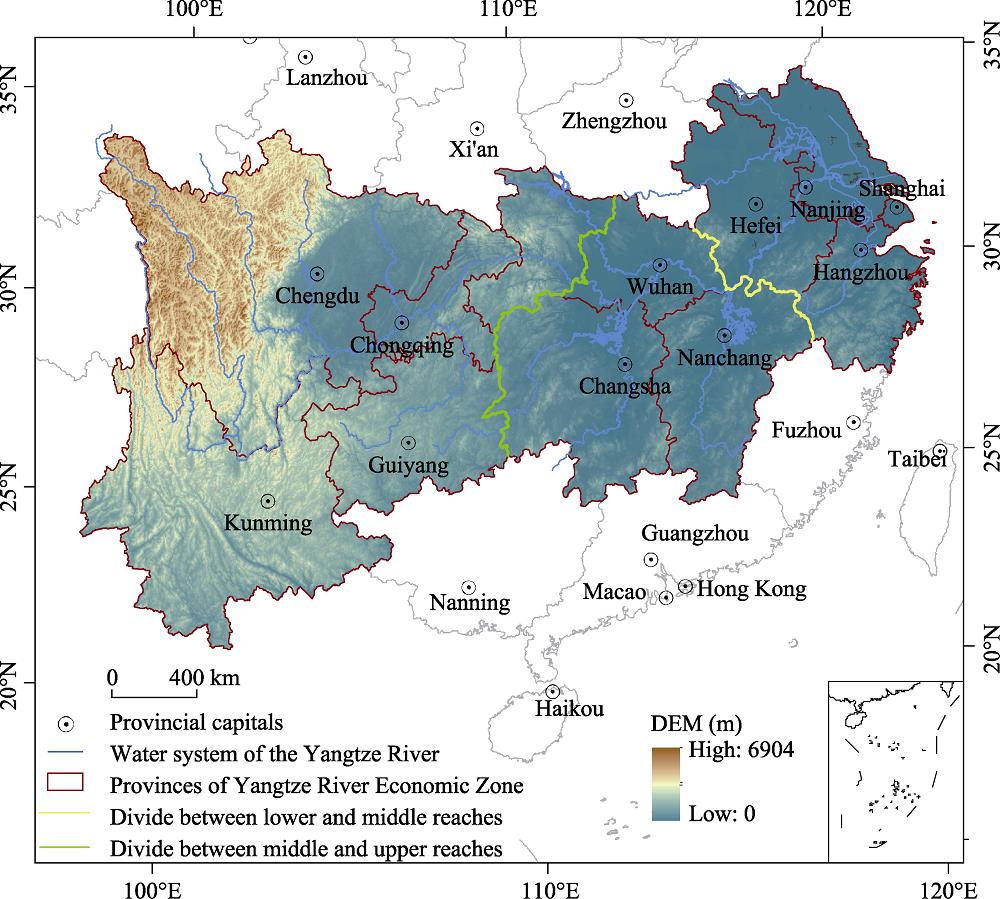
The YREZ covers 11 provincial-level regions according to the Outline for the Development Plan of the YREZ, including Shanghai, Jiangsu, Zhejiang, Anhui, Jiangxi, Hubei, Hunan, Chongqing, Sichuan, Yunnan, and Guizhou (Figure 1), with an area of ​​about 2.05 million km². Both the gross domestic product (GDP) and population of the YREZ exceed 40% of China's total respectively, hence it is one of the regions with the strongest comprehensive strength and the most strategic support in the country. Currently, the YREZ has a total of 129 prefecture-level cities (autonomous prefectures), of which, four are sub-provincial cities and two are municipalities. Among them, Qianjiang, Tianmen, Xiantao and three other cities belong to Hubei Province, the administrative level is the sub-prefecture- level city; the Shennongjia Forest Area is a county-level forest area, which belongs to Shiyan City. Note that in order to facilitate the study and to ensure the spatial integrity of the study area, this paper also sets the three sub-prefecture-level cities (e.g. Qianjiang) as independent research units and merges the Shennongjia Forest Area into Shiyan City so as to fall into the category of the YREZ. There are a total of 129 cities in the YREZ, which are taken as the research unit in our study.

We selected 2000, 2005, 2010, and 2015 as the investigated years. The relevant data required for the research are derived from: China Urban Statistical Yearbook, China Energy Statistical Yearbook, China Industrial Statistical Yearbook, China Labor Statistical Yearbook, China Environmental Statistical Yearbook, China Demographic Yearbook, 11 provinces and cities statistical yearbooks and statistical bulletins and the China Economic and Social Big Data Research Platform (http://data.cnki.net/Yearbook). The vector data of the administrative divisions of the YREZ used in the article are all from the National Basic Geographic Information Center of the People's Republic of China (http://ngcc.sbsm.gov.cn) and used in spatial analysis of subsequent articles. We use DEA-SOLVER-PRO12.1, ArcGIS10.1, Geoda1.8.10, EViews and Excel to process, transform and analyze these data.

Constructing a reasonable input-output index system is the premise and basis for objectively evaluating regional eco-efficiency. Based on the previous summaries and research results, we established an evaluation index system for regional eco-efficiency (Table 1).

In order to consider the problem of undesired output, Tone (2002) proposed a non-radial, non-angled eco-efficiency evaluation model based on the slack-based measure and data envelope analysis model in 2002.

The SBM model is used to measure the eco-efficiency, which can effectively reflect the real situation and is in line with the needs of the actual situation. Furthermore, the model can effectively avoid the deviation and impact of the radial and angular problems in the efficiency measurement.

The model is expressed as:

where ρ is the efficiency value; N, M and I represent the number of input, desired output and undesired output, respectively; ($s_{n}^{x}$,$s_{m}^{y}$,$s_{i}^{b}$) represents the relaxation vector of input, desired output and undesired output; ($x_{{k}'n}^{{{t}'}}$,$x_{{k}'m}^{{{t}'}}$,$b_{{k}'i}^{{{t}'}}$) represents the input-output value of the k° decision-making unit during the t° period; z^t_k represents the weight of the decision-making unit. The objective function ρ (0<ρ≤1) strictly monotonically decreases with respect to ($s_{n}^{x}$,$s_{m}^{y}$,$s_{i}^{b}$). When ρ = 1, the decision unit is located on the efficiency frontier and is completely valid; when ρ<1, the decision unit is a loss of efficiency. We can improve eco-efficiency by optimizing input-output relationships.

3.3.1 Global spatial autocorrelation calculations

We use the global Moran's I index as a formula to measure the similarity of eco-efficiency levels in adjacent areas:

where x_i is the observed value of region i; n is the number of observations; $\bar{x}=\frac{1}{n}\sum{_{\text{i=1}}^{n}}{{x}_{i}}$, ${{\sigma }^{2}}=\frac{1}{n}\sum{_{\text{i=1}}^{n}}{{({{x}_{i}}-\bar{x})}^{2}}$. The spatial weight matrix is w_ij. Equation (3) presents the Z test statistic:

where E(I) is the desired value, Var (I) is the variance and the value of I ranges from -1 to 1. If I is significantly positive, it indicates that there is a positive spatial correlation and the region with high (low) regional eco-efficiency value is spatially agglomerated. When I > 0, it means that the high-high value areas gathered together, and the low-low value areas also gathered together. The larger I is, the smaller the spatial space difference is. When I < 0, it suggests that the high-value and the low-value areas are clustered together, which belongs to spatial negative correlation. The smaller I is, the larger the spatial space difference is. When I = 0, the attribute value is randomly distributed in space. The Moran's index usually uses a two-sided test and the Z test (Equation 3).

3.3.2 Local spatial autocorrelation calculations

The global spatial autocorrelation assumes that the space is homogeneous and cannot reflect the local agglomeration characteristics. Hence, local spatial autocorrelation analysis is needed.

The local Moran's index is calculated as:

where I_i is Local Moran's index for the region i; Z_i is regional eco-efficiency for a standardized area i; W_ij indicates spatial weight matrix. Local Moran's index with a positive (negative) value implies that the elements of the similar (different) type attribute values ​​are adjacent, and a larger absolute value indicates a higher degree of proximity. The scatter plot is an observed corresponding spatial lag factor w_Z. A scatter plot of the ordinate reveals the intrinsic relationship between the elements of each region, with spatial neighbors being 1 and not adjacently being 0, and it has 4 types: high-high gathering, low-low gathering, low-high gathering and high-low gathering.

3.3.3 Standard deviation ellipse calculations

Welty Pfeiffer (a professor of sociology from the University of Southern California,) proposed the “Standard Deviation Ellipse” in 1926 where he expounded a common method to measure the trend of a set of points or regions and the method calculated the standard distances at the directions of x and y, respectively (Zhao et al., 2009). The two measurements can be used to define an axis of an ellipse containing the distribution of all the elements. The method calculates the standard deviation of the x-coordinate and the y-coordinate from the average center as a starting point and thereby defines the axis of the ellipse, and thus the ellipse is called a standard deviation ellipse. This ellipse can be used to measure the direction and distribution of attributes accurately (Zhao and Zhao, 2014). Its expression is:

where x_i and y_i are the spatial position coordinate of each feature. $\bar{X}$and $\bar{Y}$are the arithmetic average center, SDE_x and SDE_y are the centers of the final calculated ellipse. Then we determine the direction of the ellipse based on the X-axis, and the north (12 o'clock direction) is 0 degrees (clockwise rotation), the formula is expressed as follows:

where θ, σ_x and σ_y are the corner of the ellipse, the length of the ellipse on the X-axis, and the length on the Y-axis, respectively. The long semi-axis of the ellipse indicates the direction of data distribution and the short semi-axis is the range of data distribution. The larger the difference between the length and the half-axis (the larger the flatness), the more obvious the directivity of the data is. On the contrary, if the lengths of the semi-axes are closer, the directionality is less obvious, and it equals to a circle when the long and short axes are completely equal. The circle means that there is no directional feature, and the long and short half axes represent the range of data distribution. The shorter the length and the half-axis are, the more obvious the centripetal force of the data is presented; otherwise, the longer the length and the half-axis are, the more discrete the data is.

We set the regional eco-efficiency of the YREZ as the evaluation object of Data Envelopment Analysis (DEA), in which every city (a total of 129) was considered as a decision-making unit of DEA. Each decision-making unit had a common input-output index which was obtained through the calculation of regional cities' eco-efficiency value (Table 2). We classified the Regional Eco-efficiency Level according to previous literature and the principle of hypothesis testing method in statistics (Xu, 2009). We divided the regional eco-efficiency level into five classes (Table 3).

4.1.1 Changes of eco-efficiency at the prefecture cities scale

We encoded H1-H129 for 129 DEA decision units to facilitate the software to process the data. Combined with Table 3, Figures 2 and 3, we found that changes in the eco-efficiency value of the decision-making unit during the study period had experienced a periodic fluctuation growth trend on the time scale and space distinction.

At the time scales, there were 10 fully effective DEA cities in Guang'an, Yongzhou, Hefei, Shanghai, etc., which accounted for 7.8% of the total number. Moreover, many decision-making units had problems of regional eco-efficiency loss and low levels of efficiency. A total of 16 prefecture cities showed they were fully effective in 2005, accounting for about 12.4% of the total, which was an increase compared with 2000; 8 cities were fully effective in 2010, accounting for 6.2% of the total, which was a reduction when compared with 2005; 20 cities were fully effective in 2015, accounting for 15.5% of the total, which was an increase when compared with 2010. From 2000 to 2015, most prefecture cities had fully effective regional eco-efficiency and were located in the downstream areas and showed a fluctuating growth trend. The number of relatively effective and high-level cities had increased, most of which are distributed in the downstream; medium and medium-high levels were higher than the lower-level cities in total and most of these were concentrated in the middle and upper reaches, while the low-level cities are mostly located in the upper reaches. Overall, regional eco-efficiency levels differed highly in spatial distributed patterns.

In summary, the regional eco-efficiency was generally in a volatile rising trend from 2000 to 2015. It was in a rising trend period from 2000 to 2005, and the average value increased from 0.29 to 0.45. From 2005 to 2010, there was a downward trend with an average value decreasing from 0.45 to 0.27. There was a sharp upward trend between 2010 and 2015, with the average value rising from 0.27 to 0.50. The study years of 2000, 2005, 2010 and 2015, represent the “Ninth Five-Year Plan”, “Tenth Five-Year Plan”, “Eleventh Five-Year Plan” and “Twelfth Five-Year Plan” of China's national economic and social development, respectively. During the planning period, the development of each “five-year plan” is different and there are significant local differences and overall imbalance. The obvious changes were evident from the “Ninth Five-Year Plan” to the “Twelfth Five-Year Plan” where the relatively high areas of the lower reaches of the Yangtze River gradually expanded to the middle and upper reaches and the low-value areas decreased.

4.1.2 Changes of eco-efficiency at the provincial scale

Figure 4 shows that the eco-efficiency value ​​of 11 provinces and cities had changed greatly over different periods. The whole studied area was in the stages of rising phase fluctuations, showing an “N-shaped” distribution with an imbalanced pattern, and the provincial differences were large. As shown in Figure 5, Shanghai was fully effective at DEA for the four selected years. In 2000, the provinces and cities with relatively high regional eco-efficiency were principally Zhejiang and Jiangsu; the provinces and cities with medium to high levels eco-efficiency were Hubei and Anhui; the provinces and cities with medium to low levels eco-efficiency were Sichuan, Yunnan, Guizhou, Chongqing, Hunan and Jiangxi. In 2005, the relatively effective provinces were Zhejiang, Jiangsu and Hunan; the high-level provinces changed from Anhui (in 2000) to Hubei; the medium to medium-high levels were Anhui, Jiangxi, Chongqing, Guizhou, Sichuan, and Yunnan; no low-level areas were detected. In 2010, there was a certain fluctuation in regional eco-efficiency, the overall average was low, and there were no relatively effective areas; Zhejiang Province was the only high-level area, and barely made it into this level; Chongqing and Jiangsu were medium- to high-level areas; Hubei and Hunan were medium-level areas; and the low-level areas were Sichuan, Guizhou, Yunnan, Anhui, and Jiangxi. In 2015, the only region with a relatively effective area of eco-efficiency was Hubei; Zhejiang and Jiangsu were high-level areas; Chongqing, Hunan, and Guizhou were the medium to high-level areas; Sichuan, Yunnan, Jiangxi and Anhui were the medium-level areas; low-level areas decreased.

4.1.3 Changes in eco-efficiency in different reaches

Based on the previous results, we analyzed the eco-efficiency of different reaches in the YREZ. The regional eco-efficiency of the YREZ had significant regional differences, i.e. the distribution in the upper, middle and lower reaches was uneven (Figure 6), with certain volatility, and the overall level needs to be improved. The downstream region had the highest eco-efficiency, the average was higher than the overall average, and was far ahead of the middle and upper reaches. Among them, the eco-efficiency of Shanghai in the different periods ranked first with higher mean levels than the other regions. The increase of the eco-efficiency level in the downstream region was mainly attributed to the contribution of the efficient allocation of various input and agglomeration factors to the eco-efficiency. The downstream regions had superior geographical positions and developed economies, relatively advanced technologies and rich management experience, which could attract foreigners to invest, which in turn would attract more talent which would promote the improvement of eco-efficiency. The increase in eco-efficiency of the upper and middle reaches was relatively small, and both show lower than the average level of overall eco-efficiency growth. This may be attributed to a relatively closed location and a backward level of economic development which makes it difficult to obtain funding support for technological progress and these areas were prone to “high energy consumption, poor efficiency, and high pollution”. In this regard, we should pay close attention to the technological progress and innovation of the upper and middle reaches and improve the policy environment of technological advancement.

4.2.1 Global spatial autocorrelation

Table 4 illustrates that the global Moran's index I value ​​of eco-efficiency in different periods had passed the 5% significance test, which showed significant global autocorrelation and certain volatility in growth trend. In 2010, Moran's index I reached a maximum of 0.57. The eco-efficiency level of each decision-making unit was not randomly distributed in spatial geography. The decision-making units with similar eco-efficiency levels were affected by the flow of various elements and these units clustered in geographical distribution. Although Moran's index I both increased and decreased, on the whole, the growth trend was still greater than the relative weakening trend.

4.2.2 Local spatial autocorrelation

The eco-efficiency Moran's index I scatter plot is primarily used to identify the relationship between the various regions of the decision-making unit and the eco-efficiency levels of its adjacent regions. Its four quadrants represent four different types of spatial agglomeration mode, wherein, if the decision unit falls in the first and third quadrants, it belongs to the positive spatial autocorrelation; if the decision unit falls in the second and fourth quadrants, it is a negative spatial autocorrelation. As shown in Figure 7 and Table 5, most of the decision-making units in different periods were mainly concentrated in the first and third quadrants, showing positive spatial autocorrelation distribution characteristics. Only a few decision-making units fell into the second and fourth quadrants. These regions deviated from the local positive overall trend of spatial autocorrelation and their eco-efficiency was atypical.

From the viewpoint of various agglomeration areas, the regional eco-efficiency of different periods was clearly different. There were large differences in the distribution of high-high concentration areas in different periods. In 2000, there were 39 prefectures and cities, accounting for 30.2% of the total. In 2005, the total number of prefectures and cities decreased, with 33 prefectures, accounting for 25.6% of the total. The number continued to decrease in 2010; only 27 prefectures and cities were high-high concentration areas, accounting for 20.9% of the total. In 2015, it increased significantly and reached 40 prefectures and cities, accounting for 31.0% of the total; the low-low concentration areas in different periods are larger in terms of total proportion or overall change. The total number of prefectures and cities had decreased from 67 in 2000 to 61 in 2005 but in 2010, this increased to 76. In 2015, the total number of prefectures and cities was the same as in 2000, and it was spatially distributed and nonadjacent to other agglomeration areas; the increased or decreased distributions of the total number of low-high and high-low agglomeration areas were related to the distributed patterns of high-high agglomeration areas. Shanghai appeared in two high-low agglomeration areas, indicating that the eco-efficiency levels in Shanghai's surrounding areas in 2005 and 2010 were large and could not form high-high agglomeration areas, and low-high agglomeration areas were basically distributed in areas of high agglomeration.

Around the district, many low-concentration areas such as Kunming, Taizhou (Zhejiang), and Ningbo were stable. They were the low agglomeration areas in different periods and had not changed to high-concentration areas. The reason is that most of the cities in the area produced a diffusion effect on the surrounding area. For urban changes of each agglomeration area, the regional eco-efficiency level had obvious agglomeration and liquidity. From 2000 to 2015, the most commonly related types of adjacent cities and their adjacent areas maintained the same level, which accounted for 51.9% of the total, indicating that most cities and their adjacent cities had a high degree of spatial stability.

We found that only four cities passed the 0.1% significance level test in 2000 and 17 cities passed the 1% significance level test, including Huai'an, Zhangzhou, Taizhou (Jiangsu), 37 cities (such as Lianyungang and Hefei) passed the 5% significance level. In general, the number of cities with high-concentration areas accounted for 22.5% of the total in 2000, but less than the proportion of low accumulation areas in the total. In 2005, only Shanghai and Nantong were located in the high-concentration areas and passed the 0.1% significance level; the cities with 1% significance level were Ningbo, Chizhou, Bozhou, Suzhou (Jiangsu) and Yiyang; 12 prefectures, such as Wenshan passed the 5% significance level test; in 2005, the eco-efficiency level of YREZ was not high and needed to be improved. In 2010, there were 6 prefectures, including Nantong and Taizhou (Jiangsu), which passed the 0.1% significance level test, all of which were located in high-concentration areas; 7 cities, including Shanghai and Suzhou (Jiangsu), passed the 1% significance level. Among the 18 significant cities, such as Dali, Liangshan, Liupanshui, Guiyang, and Qiandongnan, only Yancheng, Yangzhou, Ningbo, and Enshi were in high-high concentration areas, and the rest were in low-low concentration areas. In 2015, the regional eco-efficiency was tested by the 0.1% significance level and included Nantong and Taizhou (Jiangsu). Among them, Nantong, Taizhou (Jiangsu) and Shanghai were in the high concentration area; 15 prefectures and cities, such as Zhenjiang and Suzhou (Jiangsu), were tested by the 1% significance level. The number of cities with high-high concentration areas exceeded the number of low-low concentration areas, accounting for 13.2% of the total; the number of cities with the 5% significance level was 23 and included Qianjiang and Jingzhou; the total number of those in high-high gathering areas increased to 17.8% compared with the year 2010 (Figures 8 and 9).

It can be seen that during the study period, the area of ​​the YREZ had a high eco-efficiency and a large concentration area, but the distribution was relatively concentrated, and most of them were distributed in the middle and lower reaches. Many low-low agglomeration areas were distributed in the middle and upper reaches of the Yangtze River, but the concentration was not obvious. With the passage of time, the low-low agglomeration areas gradually decreased, and high-low agglomeration areas began to emerge, resulting in the increasingly uneven regional eco-efficiency. In the case of spatial autocorrelation, the number of insignificant regions was the largest, indicating that these decision-making units and their surrounding areas were relatively low in eco-efficiency and slow in development (Figures 8 and 9).

4.2.3 Directional distribution

The standard deviation ellipse of different periods becomes the center of gravity and the standard deviation ellipse calculation results of the eco-efficiency of the YREZ are shown in Figures 10, 11 and Table 6. The standard deviation ellipse distribution range map of the eco-efficiency showed a northeast-southwest distribution pattern. This trend weakened over the years and tended to be scattered on the long semi-axis direction. The southwestern end was mainly located at the junction of Guizhou and Sichuan provinces. The easternmost and northernmost reaches reached the Yangtze River Delta and covered the entire middle and lower reaches of the Yangtze River. In the direction of the main axis, the main long axis is longer, which is quite different from the auxiliary axis, suggesting that the high-value areas of eco-efficiency were mainly distributed in the northeast-southwest. There was an obvious polarization. The standard distance of the main shaft increased from 848,975.7 m in 2000 to 872,024.5 m in 2015, indicating that the eco-efficiency was scattered in the northeast-southwest distribution pattern, and the standard distance of the auxiliary shaft reduced 5679.7 m from 2000 to 2015, which indicated that the eco-efficiency of this period had a polarization trend on the short axis; the corner has decreased from 69.4° in 2000 to 68.6° in 2005, and this distribution trend had increased, mainly due to Yunnan which is located in the southwest. The eco-efficiency level of Guizhou had increased from 2005 to 2015 and the corner also increased, which could be attributed to the decreased eco-efficiency values ​​of Anhui and Jiangsu provinces.

For the diffusion path of gravity, the eco-efficiency center was primarily located in the central part of Hubei (29.55°-30.43°N, 113.09°-115.47°E), i.e. the center of gravity was Huanggang in 2000, Jingzhou in 2005, Ezhou in 2010 and on the border of Jingzhou and Xiantao in 2015. The center of gravity moved to the southwest by a distance of 255.2 km from 2000 to 2005, the center of gravity moved to the northeast by a distance of 178.5 km from 2005-2010, and the center of gravity moved to the southwest by a distance of 178.5 km from 2010-2015. All in all, the change of gravity within 300 km was located in the middle reaches of the Yangtze River and underwent an alternating evolution process from northeast to southwest.

This process was reduced by the eco-efficiency of Sichuan, Yunnan, Chongqing and Guizhou. The increase-decrease-increase trend was consistent, indicating that the center shift was mainly controlled by the increase and decrease of the eco-efficiency of Sichuan, Yunnan, Chongqing and Guizhou provinces.

Based on the SBM-DEA model, spatial autocorrelation and standard deviation ellipse of undesired output, we set 129 geodesic cities in the YREZ as research units in 2000, 2005, 2010 and 2015. The regional eco-efficiency level and spatial pattern evolution characteristics were analyzed. Results show that:

The overall change of regional eco-efficiency in the YREZ is large and irregular, especially at the provincial scale, with an “N-shaped” and uneven distribution. For prefectures and cities, regional eco-efficiency periodically fluctuates at the time scale and there are discrepancies at the spatial scales. On the basin scale, the regional eco-efficiency value of the lower reaches is the largest and is the smallest in the upper reaches.

The global autocorrelation values ​​of regional eco-efficiency have passed the 5% significance test during the study period and show a certain volatility in the growth trend, indicating the efficiency levels of ecological factors of the decision-making units in the YREZ are not randomly distributed in spatial geography, they have significant effects on each other and have shown a certain aggregation effect. In terms of local spatial autocorrelation, the eco-efficiency of each cluster area is significant in different periods, with obvious aggregation and liquidity forming some high-high concentration areas which are centered on Shanghai and surrounding cities, with low-low clusters centered on the cities of the middle and upper reaches. With the study period changes, the spatial distribution of the decision-making units also changes, and the amplitude is large, whereas, only a few prefectures and cities with low-high aggregation zones and high-low polarization agglomeration zones do not form a certain distribution range. In terms of direct distribution, the regional eco-efficiency value shows the spatial distribution pattern in the northeast-southwest direction. The regional eco-efficiency shows the evolution pattern from northeast to southwest in different research periods. On the other hand, we analyze the regional eco-efficiency impact mechanism by constructing a spatial econometric model. Research suggests that the regional eco-efficiency of the YREB is mainly influenced by economic development level, industrial structure, scientific and technological strength, human capital, environmental regulation and other factors (all of these pass the significance test). Among these, industrial structure is the most influential factor; human capital is limited by the level of education per capita and has the least impact. We also give some policy recommendations based on research conclusions. “With respect to different influencing factors, each region must change its regional development model, and clarify its own lack of development and apply the right medicine to improve regional eco-efficiency, break down administrative barriers between cities in the region, establish a cross-regional coordinated development mechanism, and jointly build a shared watershed ecological community, and eventually realize the coordinated and sustainable development of the YREB.”

In summary, this paper believes that the regional eco-efficiency level of the YREZ is mainly affected by factors such as economic development level, industrial structure, scientific and technological strength, human capital, environmental regulation, etc. In order to improve regional eco-efficiency of the YREZ and break down inter-regional city administrative barriers, establish a cross-regional coordinated development mechanism, and jointly build a shared watershed ecological community, all regions must change their regional development patterns, clarify their own deficiencies and finally achieve coordinated and sustainable economic development strategies.

References

[1] Eco-efficiency for sustainable manufacturing: An extended environmental costing method. Production Planning and Control, 23, 134-144(2012).
[2] Material flow and energy flow in iron and steel enterprises and their relationship. Journal of Natural Science, 27, 979-982(2006).
[3] Eco-efficiency evaluation of the petroleum and petrochemical group in the map Ta Phut Industrial Estate, Thailand. Journal of Cleaner Production, 19, 241-252(2011).
[4] Empirical analysis of regional ecological efficiency evaluation and influencing factors in China: Taking interprovincial data from 2000 to 2006 as an example. Chinese Management Science, 16, 566-560(2008).
[5] Measuring eco-inefficiency: A new frontier approach. Operations Research, 60, 1064-1079(2012).
[6] Research on total factor energy efficiency of Chinese manufacture industry and its influence factors based on SFA. China Soft Science Magazine, 180-192(2014).
[7] Economic efficiency, environmental efficiency and eco-efficiency of the so-called two vertical and three horizontal urbanization areas: Empirical analysis based on HDDP and Co-Plot method. The Empirical Chinese Soft Science, 96-109(2015).
[8] et alMaterial input and output analysis of Chinese economy system. Acta Scientiarum Naturalium Universitatis Pekinensis, 39, 538-547(2003).
[9] Eco-efficiency trends in the UK steel and aluminum industries. Journal of Industrial Ecology, 9, 171-188(2005).
[10] Research on regional ecological efficiency based on three-stage DEA model. China Soft Science, 92-99(2011).
[11] Cleaner production, eco-industrial and circular economy. Environmental Science Research, 14, 1-4(2001).
[12] Determination of evaluation indicators of China’s regional industrial eco-efficiency and DEA analysis. China Population, Resources and Environment, 21, 318-321(2011).
[13] National environmental pressure indicators and dematerialization analysis. Shenyang: Northeastern University(2005).
[14] A conditional directional distance function approach for measuring regional environmental efficiency: Evidence from UK regions. European Journal of Operational Research, 227, 182-189(2013).
[16] Research on regional environmental efficiency difference and evolution law in China: Analysis of SBM Model based on unexpected output. Journal of Industrial Technological Economics, 27, 100-104(2008).
[17] Examining the drivers of total factor productivity change with an illustrative example of 14 EU countries. Ecological Economics, 72, 60-69(2011).
[18] et alRegional eco-efficiency indicators: A participatory approach. Journal of Cleaner Production, 14, 1603-1611(2006).
[19] Eco-efficiency of the world cement industry: A data envelopment analysis. Energy Policy, 39, 2842-2854(2011).
[20] Agricultural eco-efficiency evaluation in China based on SBM model. Acta Ecologica Sinica, 33, 3837-3845(2013).
[21] Evaluation of regional ecological efficiency and its spatial econometric analysis. Resources and Environment in the Yangtze River Basin, 22, 640-647(2013).
[22] What is energy efficiency? Concepts, indicators and methodological issues. Energy Policy, 24, 377-390(1996).
[23] Urban ecological footprints: Why cities cannot be sustainable: And why they are a key to sustainability. In: Urban Ecology. Boston: Springer(2008).
[26] A strange case of the cost and allocative efficiencies in DEA. Journal of the Operational Research Society, 53, 1225-1231(2002).
[27] Communicating the eco-efficiency of products and services by means of the eco-costs/value model. Journal of Cleaner Production, 10, 57-67(2002).
[28] National Footprint and Biocapacity Account 2005: The Underlying Calculation Method. Oakland, CA, USA: Global Footprint Network(2005).
[29] Perceptual and structural barriers to investing in natural capital: Economics from an ecological footprint perspective. Ecological Economics, 20, 3-24(1997).
[30] Study on regional industrial eco-efficiency in China based on DEA theory. Ecological Economy, 24-28(2011).
[31] Assessment for eco-efficiency of China’s textile industry based on material metabolism. China Population, Resources and Environment, 18, 116-121(2008).
[32] Research on total factor energy efficiency of China manufacture empirical analysis based on 28 sectors. Modern Economic Science, 20-25(2010).
[33] Energy efficiency and its influencing factors: Based on the positive analysis of DEA. Management World, 66-76(2007).
[34] Seven energy efficiency indicators and their measurement approaches. China Soft Science, 128-137(2010).
[35] The eco-efficiency evaluation on petrochemical industry based on three-stage DEA model. Advanced Materials Research, 219/220, 1468-1471(2011).
[38] . Probability Theory and Mathematical Statistics(2009).
[39] . Half is Enough: An Introduction to Cleaner Production(2006).
[40] et alIndustrial eco-efficiency and its spatial-temporal differentiation in China. Frontiers of Environmental Science & Engineering, 6, 559-568(2012).
[41] Sustainable development index system and financing appraisal research for Chinese iron and steel enterprises based on resource utilization efficiency. Shenyang: Northeastern University(2009).
[42] Eco-efficiency analysis of industrial system in China: A data envelopment analysis approach. Ecological Economics, 68, 306-316(2008).
[43] Material flow analysis and data envelopment analysis based regional eco-efficiency analysis: Case Study of Jiangsu Province. Acta Ecologica Sinica, 29, 2473-2480(2009).
[44] Evaluation on recycle economy of Gansu province based on accounting of material flowing and eco-footprint. Lanzhou: Lanzhou University(2011).
Set citation alerts for the article
Please enter your email address
© Copyright 2018-2021 | Chinese Laser Press. All Rights Reserved 沪ICP备15018463号-20