Researching | Research on CNN Denoising Algorithm Based on an Improved Mathematical Model for the Measurement of Far-field Focal Spot

Journals >Acta Photonica Sinica >Volume 49 >Issue 12 >Page 118 > Article

Acta Photonica Sinica
Vol. 49, Issue 12, 118 (2020)

Research on CNN Denoising Algorithm Based on an Improved Mathematical Model for the Measurement of Far-field Focal Spot

Zheng-zhou WANG, Li WANG, Meng TAN, Ya-xuan DUAN^*, Wei WANG, Xin-feng TIAN, and Ji-tong WEI

Author Affiliations

Xi'an Institute of Optics and Precision Mechanics， Chinese Academy of Science， Xi'an710119， China

show less

DOI: 10.3788/gzxb20204912.1212001 Cite this Article

Zheng-zhou WANG, Li WANG, Meng TAN, Ya-xuan DUAN, Wei WANG, Xin-feng TIAN, Ji-tong WEI. Research on CNN Denoising Algorithm Based on an Improved Mathematical Model for the Measurement of Far-field Focal Spot[J]. Acta Photonica Sinica, 2020, 49(12): 118 Copy Citation Text

show less

Schematic diagram of the measurement for far-field focal spot using schlieren method

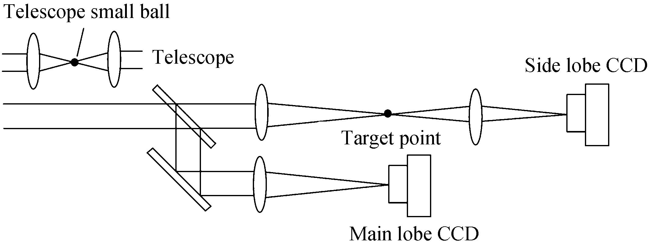
Fig. 1. Schematic diagram of the measurement for far-field focal spot using schlieren method

Download full size | View in the Article

Schematic diagram of reconstructed area using schlieren method

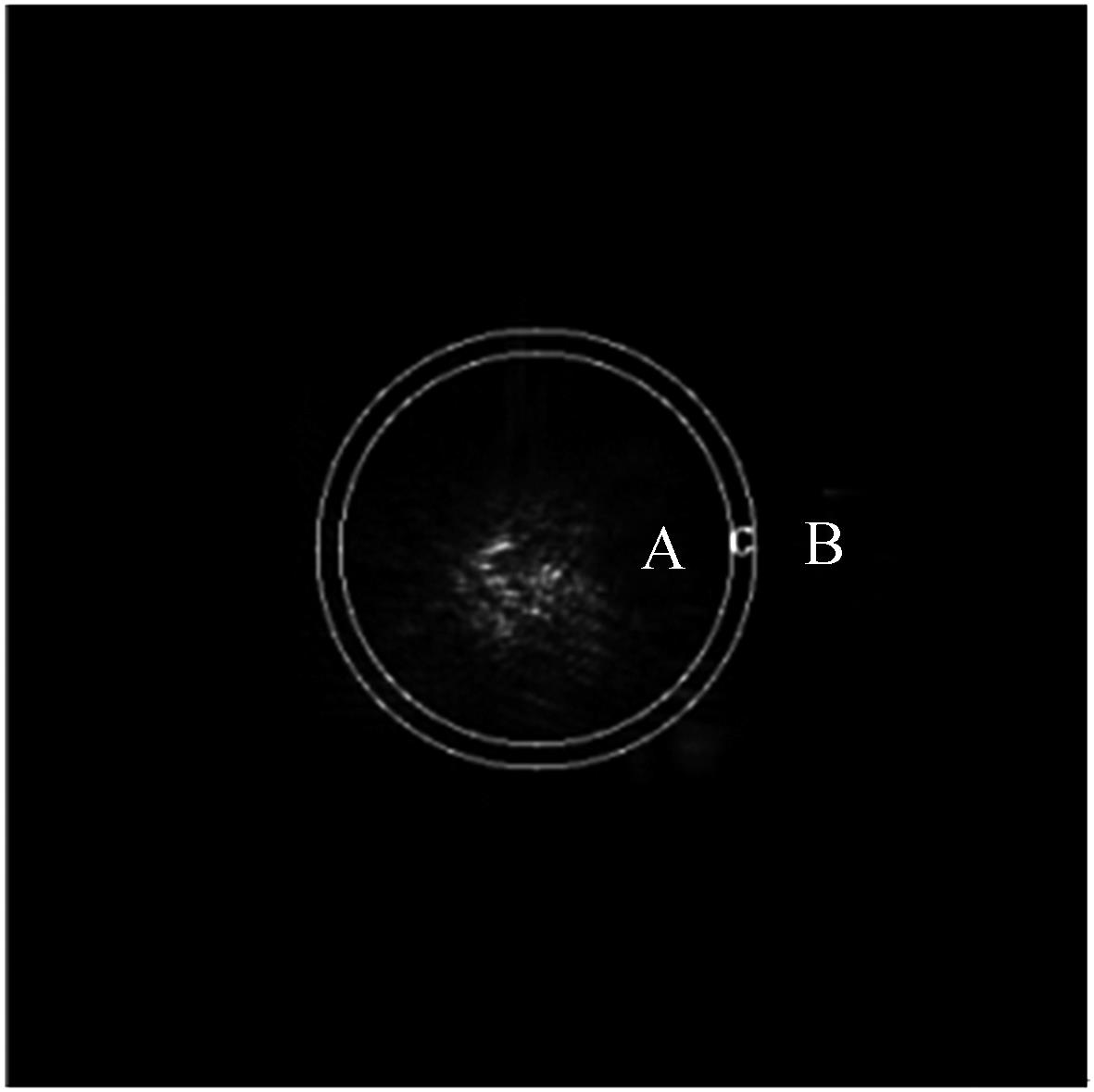
Fig. 2. Schematic diagram of reconstructed area using schlieren method

Download full size | View in the Article

Fig. 3. Data processing flow chart

Download full size | View in the Article

Fig. 4. The initial experimental data obtained by simulation parameters

Download full size | View in the Article

Fig. 5. The original image

Download full size | View in the Article

Fig. 6. Experimental data preprocessing

Download full size | View in the Article

Fig. 7. The denoising images of mainlobe beam and sidelobe beam

Download full size | View in the Article

Fig. 8. The reconstructed image of far-field focal spot

Download full size | View in the Article

Fig. 9. The denoise effect of DnCNN algorithm

Download full size | View in the Article

Fig. 10. Comparison between mainlobe and sidelobe image denoising effect (y = 256 curve)

Download full size | View in the Article

Fig. 11. Dynamic range analysis of measurement for far-field focal spot

Download full size | View in the Article

Fig. 12. Comparison of denoising effects of DnCNN on different noise levels

Download full size | View in the Article

Fig. 13. The accuracy analysis of reconstructed focal spot

Download full size | View in the Article

Fig. 14. Comparison of logarithm function curve between original image and reconstructed image y=256

Download full size | View in the Article

Fig. 15. Optical schematic of integrated diagnostic system of host device

Download full size | View in the Article

Fig. 16. The comparison of denoising results between mainlobe image and sidelobe image

Download full size | View in the Article

Fig. 17. The merged image using real captured image

Download full size | View in the Article

Fig. 18. Feature analysis of splicing area

Download full size | View in the Article

No.	Parameter	Name	Value	Unit
1	$λ$	The central wavelength of laser	6.3500×10^－4	mm
2	a	The radius of the measured hole	0.5	mm
3	f	The focal length of telecentric lens	100	mm
4	Am	The magnification	1	mm
5	pixel	The size of pixel	0.005 6	mm

Table 1. Experiment parameters for laser intensity distribution of far-field focal spot

View in the Article

No.	MSE	PSNR	Correlation coefficient		Energy integral ratio between Org. and De. curve (y=256)	Error between Org. and De. curve (y=256)
No.	MSE	PSNR	Org. and De. image	Org. and De. curve(y=256)	Energy integral ratio between Org. and De. curve (y=256)	Max	Min	Mean
1	5	22.15	0.996 0	0.998 2	0.961 9	56.23	-23.77	-3.62
2	10	24.24	0.995 8	0.998 1	0.962 7	57.96	-24.43	-3.74
3	25	25.17	0.995 3	0.997 8	0.964 1	59.49	-26.61	-3.87
4	50	29.23	0.994 4	0.997 1	0.969 6	48.26	-34.59	-4.25
5	100	33.39	0.985 0	0.980 9	1.089 8	61.83	-96.30	-5.67
6	200	34.70	0.722 2	0.803 3	1.109 2	285.5	-413.9	-13.43

Table 2. Comparison of denoising effects of DnCNN on different noise levels

View in the Article

		Org. Max (y=256)	Merge Max (y=256)	Error of log10 curve	Error of gray curve	Dynamic range
		Org. Max (y=256)	Merge Max (y=256)	Error of log10 curve	Error of gray curve	Is used	Org. Image	Merge Image	Error
Mainlobe		$C_{m a x}^{}$ =5.855 4	$M_{m a x}^{}$ =5.848 1	-0.007 3	11 864	Yes	1 286.3	1 328.9	3.22%
Side lobe	Peak 1	$S_{m a x}^{1}$ =4.091	$M_{m a x}^{1}$ =3.904	0.187 0	4 314	No
	Peak 2	$S_{m a x}^{2}$ =3.474	$M_{m a x}^{2}$ =3.184	0.290 0	1 452	No
	Peak 3	$S_{m a x}^{3}$ =3.06	$M_{m a x}^{3}$ =3.056	0.0040	11	No
	Peak 4	$S_{m a x}^{4}$ =2.746	$M_{m a x}^{4}$ =2.725	0.0210	26	Yes

Table 3. The error comparison of dynamic range of reconstructed focal spot

View in the Article

	Diagnostic perspective	Diffraction limit	Wavelength of laser beam	Dynamic range	CCD type
Mainlobe CCD	185 μrad	38 times	351 nm	100∶1	12 bits and scientific level
Sidelobe CCD	150 μrad~600 μrad	30~120 times	351 nm	100∶1	12 bits and scientific level

Table 4. The experimental parameter of focal spot of far-field

View in the Article

No.	Denoising method	Denoising function	The correlation coefficient between original image and reconstructed image
1	Random noise estimation method	rand2	0.994 5
2	Minus variance method	Std2	0.968 4
3	Minus background gray	GetBack	0.989 6
4	DnCNN algorithm	DnCNN	0.998 9

Table 5. Comparison of correlation coefficient between original image and reconstructed image using different denosing method

View in the Article

Get PDF(in Chinese)

Figures&Tables (23)

References (17)

Copy Citation Text

Zheng-zhou WANG, Li WANG, Meng TAN, Ya-xuan DUAN, Wei WANG, Xin-feng TIAN, Ji-tong WEI. Research on CNN Denoising Algorithm Based on an Improved Mathematical Model for the Measurement of Far-field Focal Spot[J]. Acta Photonica Sinica, 2020, 49(12): 118

Download Citation

Save the article for my favorites

Paper Information

Recommended Topics

laser devices and laser physics

Lasers and Laser Optics

laser manufacturing

Instrumentation, Measurement and Metrology

Set citation alerts for the article

Please enter your email address