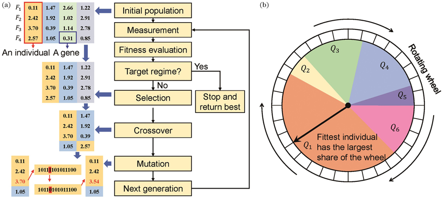
Fig. 1. Principle of genetic algorithm. (a) Genetic algorithm flowchart; (b) schematic of the “roulette wheel” selection

Fig. 2. Architectures of artificial neural network^[40]

Fig. 3. Evolutionary algorithm to implement smart mode-locking^[27]. (a) Experimental setup for locking an NPR-based MLFL through an evolutionary algorithm; (b)(c) mode-locked (b) and unstable Q-switched mode-locked regime (c) found during the run of the evolutionary algorithm fitness designed with signal intensity; (d) evolution of the average and best values of fitness function defined with radio frequency (RF) component intensity; (e)(f) temporal pulse train (e) and the optical spectrum (f) of the fundamental mode-locking regime found by the evolutionary algorithm

Fig. 4. Intelligent control of all-normal dispersion(ANDi) fiber laser^[31]. (a) Schematic of an all-normal dispersion fiber laser with liquid crystal (LC); (b) diagram of the two configurations of the LC phase retarder showing the forward (left) and backward (right) propagation directions; (c) mode-locked states found through a scan over all available voltages, showing spectra for several operating points (three control values represent spatial position and the fourth value represents the color of the marker); (d)(e) pulse duration as a function of environmental temperature in a standard oscillator (d) and an LC stabilized oscillator (e); (f) spectrum of the mode-locked ANDi laser (solid) recovered by genetic algorithm from a random starting point using a target spectrum (dashed); (g) measured FROG traces measured during the temperature cycling run with the numbers i-iv corresponding to the time and temperatures indicated in Fig. (e), where the spectral is inset in white along the appropriate axes

Fig. 5. Intelligent programmable laser based on human-like algorithm^[34]. (a) Experiment setup of intelligent mode-locked fiber laser; (b) comparison over initial lock time, recovery time and the number of mode-locking regimes between human-like algorithm and recent automatic mode-locking algorithms; (c) schematic of human-like algorithm; (d) operation regimes, from left to right respectively shows the fundamental mode-locking, the second-order harmonic mode-locking, the third-order harmonic mode-locking, the Q-switch, and the Q-switch mode-locking operation regimes

Fig. 6. Intelligent fiber laser based on deep learning algorithm^[45]. (a) Experimental setup of deep learning ultrafast fiber laser; (b) structure of the low-latency deep-reinforcement learning algorithm based on deep deterministic gradient strategy in the laser environment; (c) characterization of the output when the laser is in the fundamental mode-locking state; (d) effect diagram of algorithm recovery after the laser loses mode-locked state due to motor vibration, including the convergence curves of the reward values in the last 100 training iterations of the stable mode-locking computational model (top left), the repetition frequency and power change of the laser output during the process of applying vibration to the laser (top right), the recovery time statistics of 1500 vibration tests (down left), the output power change of the system within 10 min under the condition of vibrating for 1.5 s per minute and running the mode-locked recovery algorithm all of the time (down right)

Fig. 7. Spectral width and shape programmable fiber lasers^[35]. (a) Experiment setup diagram; (b)(c) spectral shape programming: the hyperbolic secant spectrum (b), the triangular spectrum (c); (d)-(f) spectral width programming from 10 to 40 nm, showing the spectra (d), autocorrelation traces (e), and the repeatability test for the maximum spectral FWHM (f)

Fig. 8. Multimode intelligent fiber laser^[36]. (a) Schematic diagram of a genetic multimode fiber laser using wavefront shaping; (b) power increases with the increase of generation number, where the inset shows the optimal phase map displayed on the spatial light modulator (SLM); (c) optical spectra before and after optical power enhancement; (d)-(f) mode profile cleaning of the genetic multimode fibre laser working in the quasi-CW state, where the Fig.8(d) is mode profile before genetic optimization, Fig.8 (e) is mode profile after genetic optimization, and Fig.8(f) is mode profile comparison before and after genetic optimization

Fig. 9. Sketch of RF signal under breather mode locking

Fig. 10. Dynamics of relaxation oscillation and noise-like pulse^[37]. (a)-(c) Dynamics of relaxation oscillation: (a) RF spectrum extracted by fast Fourier transform (FFT) of the relaxation oscillation temporal intensity signal, featuring many sidebands around the fundamental repetition frequency; (b) corresponding time trace of relaxation oscillation captured by the oscilloscope; (c) DFT optical spectrum evolution of the relaxation oscillation over 2000 cavity periods, where the white curve represents the energy evolution. (d)-(f) Dynamics of noise-like pulse emission: (d) RF spectrum of the output extracted by FFT of the temporal intensity signal, where the inset shows a magnified version of the sidebands; (e) corresponding time trace captured by the oscilloscope; (f) evolution of DFT optical spectrum roundtrip by roundtrip obtained by DFT, revealing the typical noisy spectrum of noise-like pulse mode locking

Fig. 11. Experimental results of the intelligent search for single breathers^[37]. (a) Evolution of the average (red circles) and maximum (blue squares) fitness function value over successive generations, for the merit function given in equation (6). (b)-(d) Characteristics of the optimized state: (b) RF spectrum obtained by FFT of the signal from the photodiode; (c) dispersive Fourier transform recording of single-shot spectra over consecutive cavity round trips (RTs), where the white curve represents the energy evolution; (d) temporal evolution of the intensity relative to the average RT time over consecutive RTs

Fig. 12. Intelligent control of breathing ratio^[37]. (a)-(c) Dynamics of breathers with small breathing ratio of 1.076; (d)-(f) dynamics of breathers with moderate breathing ratio of 1.471; (g)-(i) dynamics of breathers with large breathing ratio of 1.816; (a)(d)(g) dispersive Fourier transform recording of single-shot spectra over consecutive cavity round trips (RTs); (b)(e)(h) temporal evolution of the intensity relative to the average RT time over consecutive RTs; (c)(f)(i) single-shot spectra at the RT numbers of maximal and minimal spectrum extents within a period

Fig. 13. Genetic algorithm optimization results for breathing solitons with a tunable oscillation period^[37]. (a)(b) Dynamics of breathers with large oscillation period; (c)(d) dynamics of breathers with moderate oscillation period; (e)(f) dynamics of breathers with small oscillation period; (a)(c)(e) dispersive Fourier transform recording of single-shot spectra over consecutive RTs; (b)(d)(f) temporal evolution of the intensity relative to the average RT time over consecutive RTs

Fig. 14. Typical genetic algorithm optimization results for breather molecules^[37]. (a)-(d) Dynamic of “increasing-phase” breather molecule; (e)-(h) dynamic of “oscillating-phase” breather molecule; (a)(e) dispersive Fourier transform (DFT) recording of single-shot spectra over consecutive cavity RTs, over-dense spectral modulation causes a Moiré interference pattern in Fig.14(a); (b)(f) close-up view of the DFT recorded spectral data; (c)(g) evolution of the first-order single-shot autocorrelation trace over consecutive RTs; (d)(h) evolution of the relative phase difference between the two breathers (red curve) and the total energy of the molecule (black curve) as a function of the time

Fig. 15. RF spectral measurements of frequency-locked and frequency-unlocked breathers (the reference frequency is one-fifth of the fundamental repetition frequency)^[54]. (a)(b) Single-mode oscillation of frequency-locked breather measured over spans of 50 kHz and 100 Hz, respectively; (c)(d) multi-mode oscillation of frequency-unlocked breathers measured over 50 kHz and 10 kHz spans, respectively

Fig. 16. Change in breathing frequency over time for the frequency-locked and frequency-unlocked breathers, as measured with a cymometer. The former is 3500 times more stable than the latter, and SD means standard deviation^[54]

Fig. 17. Breathing frequency/winding number with pump power in a series of plateaus. The plateaus corresponding winding number forms the Farey tree, as shown in the inset. The winding number refers to the ratio of breathing frequency (f_b) and repetition frequency f_r; the winding number equal to 1/5 means that fb/fr equal to 1/5^[54]

Fig. 18. Experiment setup of the intelligent laser with polarization control based on liquid crystal phase delayers^[54]

Fig. 19. Machine-learning results^[54]. (a) Evolution of the mean and best fitness function value of the individuals for each generation, as well as the corresponding evolution of the SNR (signal-to-noise ratio) of the breathing frequency; (b)(c) breathing frequency is constant with the variation of pump power and polarization, showing stable optimal state (locked-frequency breather)