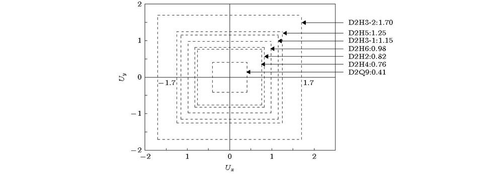
Fig. 1. Positivity analysis of lattice Boltzmann discrete models. The dash squares denote the positive areas of each lattice Boltzmann discrete model, which are constructed as . The values of each model are annotated after the model names. 格子Boltzmann离散模型正值性分析　虚线框表示模型正值区域, 其涵盖区域为 , 模型 标注在图中模型名称之后

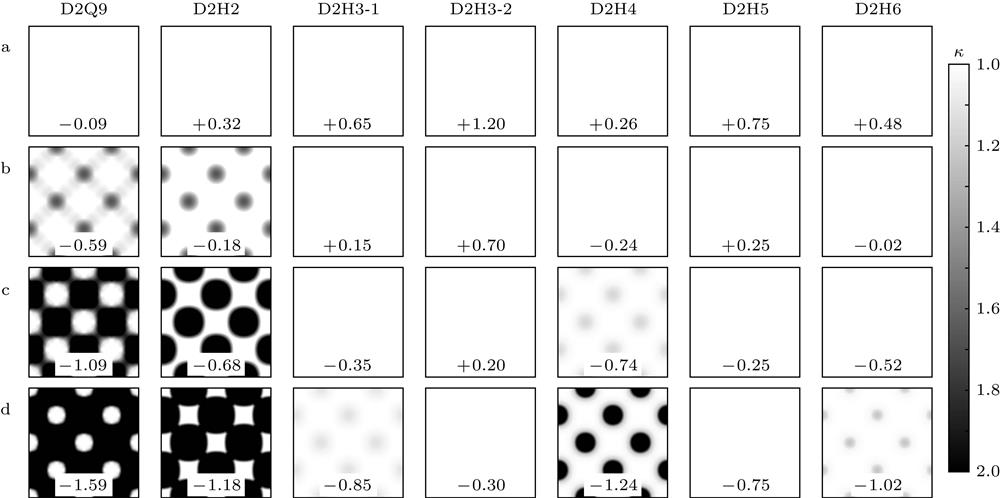
Fig. 2. The initial filled contours of designed Taylor-Green vortex simulations for each lattice Boltzmann model in the fluid domain . Each column is a simulation set of a lattice Boltzmann model with different designed cases. Each row is a set of a simulation case with different lattice Boltzmann models. The values in the contour panels are the values of , i.e. the difference between the and the designed . For the sake of identifying the positivity violation process of a lattice Boltzmann model, the filled contours truncate the range of , limiting into . 各格子Boltzmann模型在Taylor-Green涡设计计算工况下初始时刻计算流域 内 值色阶图　图中列对应格子Boltzmann模型, 行则对应表3中计算工况; 每个色阶图上方的数值 值, 即正值区域值 设计计算工况 差值;为方便观察正值性随计算工况遭到破坏的变化过程, 图中对 值做了截断处理, 仅区别 范围变化

Fig. 3. The contour lines of Taylor-Green vortex in fluid domain at half-value decay time , including the theoretical solution (denoted as “Theoretical”) and the numerical results of lattice Boltzmann models. Each column is a set of simulations under the designed cases. Each row is a set of simulations under selected lattice Boltzmann models including the theoretical solution. Taylor-Green涡半衰时刻 , 流域内, 不同计算工况下理论解(Theoretical) 与各格子Boltzmann模型的速度平方和 等高线图; 图中列对应格子Boltzmann模型, 行则对应表3中计算工况

Fig. 4. The error evolution of each simulation. The panel a, b, c, d renders each designed case in Table 3 respectively. For the sake of rendering, the unit of the time axis is scaled as 0.173286795 s. 各Taylor-Green涡设计计算工况下, 各格子Boltzmann模型计算误差随时间演变, 图中标号a, b, c, d分别对应表3各设计计算工况; 为方便表示, 图中横坐标单位为

Fig. 5. The error comparison of Taylor-Green vortex simulations with postive value of . The designed configurations of Taylor-Green vortex are denoted with line styles, in which the solid, dashed and dash-dotted line indicates case a, b and c in Table 3 respectively, meanwhile the lattice Boltzmann models are labeled with line colors and markers. For the sake of rendering, the unit of the time axis is scaled as 0.173286795 s. Taylor-Green涡设计计算工况下, 值为正值的各格子Boltzmann模型数值模拟误差对比. 图中实线, 虚线和虚点线分别为工况a, b, c (见表3)结果, 离散模型则用颜色和符号标注. 为方便表示, 图中横坐标单位为0.173286795 s

Fig. 6. The numerical performance of Taylor-Green vortex simulations vs the value of . Panel a plots the numerical errors of model D2H4 under case a, b, c and model D2H5 under case b, c, d, which possess close value of respectively. Panel b plots the numerical errors of simulations with a value of around . The numbers labeled on the curves are their values of . The simulation configurations are denoted with line style, in which solid, dashed, dash-dotted and dotted line indicates case a, b, c and d respectively, meanwhile the lattice Boltzmann models are labeled with line colors and markers. In all panels, the results of model D2H3-2 with four designed configurations are plotted for a reference. The designed configurations of Taylor-Green vortex are denoted with line styles, in which the solid, dashed, dash-dotted and dotted line indicates case a, b, c and d in Table 3 respectively, meanwhile the lattice Boltzmann models are labeled with line colors and markers. For the sake of rendering, the unit of the time axis is scaled as 0.173286795 s. Taylor-Green涡数值模拟误差与 值相关性分析　(a)对比了 接近的D2H4模型a, b, c工况与D2H5模型b, c, d工况计算误差; (b)对比了 在 附近所有数值模拟计算误差. 所有图中均保留了D2H3-2模型在a, b, c, d工况下的计算误差作为参照. 曲线上标注值为该数值模拟的 值. 图中a, b, c, d工况分别用实线, 虚线, 虚点线及点线标注, 而离散模型则用颜色和符号标注. 为方便表示, 图中横坐标单位为0.173286795 s

Fig. 7. The numerical performance of Taylor-Green vortex simulations vs initial . The error evolutions of numerical simulations with negative values of but negligible departure of initial from are plotted, including model D2H3-1 under case c, model D2H3-2 under case d, model D2H4 under case b, model D2H5 under case c,d and model D2H6 under case b, c. The results of model D2H3-2 with four designed configurations are also plotted for a reference. The designed configurations of Taylor-Green vortex are denoted with line styles, in which the solid, dashed and dash-dotted line indicates case a, b and c in Table 3 respectively, meanwhile the lattice Boltzmann models are labeled with line colors and markers. For the sake of rendering, the unit of the time axis is scaled as 0.173286795 s. Taylor-Green涡数值模拟误差与初始 值相关性分析.　图中对比了在 值为负情况下, 初始 值偏离 幅值可忽略的算例计算误差, 包括模型D2H3-1工况c, 模型D2H3-2工况d, 模型D2H4工况b, 模型D2H5工况c, d和模型D2H6工况b, c. 图中均保留了D2H3-2模型在a, b, c, d工况下的计算误差作为参照. 曲线上标注值为该数值模拟的 值. 图中a, b, c, d工况分别用实线, 虚线, 虚点线及点线标注, 而离散模型则用颜色和符号标注. 为方便表示, 图中横坐标单位为0.173286795 s

Table 1. The first five physicists′ Hermite polynomials.

Table 2. Discrete model description of lattice Boltzmann method. For the seeking of space saving, the parameters illustrated in this table are of the corresponding unidimensional models. In numerical implementations, they require tensor product illuminated in Eq. (9) and Eq. (10). It should be noted that the table lists the lattice constant c instead of the lattice sonic speed , which can be expressed as . 格子Boltzmann离散模型. 为方便展示, 表格罗列的是用于对应构造高阶模型的一维模型参数. 实际计算中需根据(9)式和(10)式对表格中的参数进行张量构造. 另外需注意的是表格中罗列的是网格常数c, 其与格子声速 存在如下换算关系

Table 3. Case design for lattice Boltzmann method