• Photonics Research
  • Vol. 10, Issue 8, 1877 (2022)
Hao Liu1、5、†,*, Shu-Wei Huang1、2、†, Wenting Wang1, Jinghui Yang1, Mingbin Yu3, Dim-Lee Kwong3, Pierre Colman4, and Chee Wei Wong1、6、*
Author Affiliations
  • 1Fang Lu Mesoscopic Optics and Quantum Electronics Laboratory, University of California Los Angeles, Los Angeles, California 90095, USA
  • 2Department of Electrical, Computer, and Energy Engineering, University of Colorado Boulder, Boulder, Colorado 80309, USA
  • 3Institute of Microelectronics, Singapore, Singapore
  • 4Université de Bourgogne Franche-Comté, ICB, UMR CNRS 6303, Dijon, France
  • 5e-mail: haoliu1991@ucla.edu
  • 6e-mail: cheewei.wong@ucla.edu
  • show less
    DOI: 10.1364/PRJ.459403 Cite this Article Set citation alerts
    Hao Liu, Shu-Wei Huang, Wenting Wang, Jinghui Yang, Mingbin Yu, Dim-Lee Kwong, Pierre Colman, Chee Wei Wong. Stimulated generation of deterministic platicon frequency microcombs[J]. Photonics Research, 2022, 10(8): 1877 Copy Citation Text show less
    Platicon pulse generation in normal-dispersion frequency combs: operating regimes, numerical modeling, and modulated pump experimental setup. (a) 2D evolution map of platicon temporal profile as a function of intracavity fast time and detuning. Four characteristic stages are selected to show the details of the evolution in panel (b). (b) Upper panels: temporal profiles of the platicon at different evolution stages; lower panels: frequency spectra corresponding to each state. (b1) Sinusoidal input (seeding); (b2) initialization of wave breaking. Self-steepening shows that wave breaking is about to happen, with modulation maxima directed outwardly and minima directed inwardly. (b3) Post-wave breaking. Wave breaking happens, and a broad square pulse is generated; (b4) a shorter narrow platicon is generated for increasing red detuning, such as at δ=+0.2531. (c) The simulated autocorrelation of the square pulse shown in (b4). The width of the triangle is twice of the width of the square pulse. (d) Schematic setup of platicon generation. The cw laser from the ECDL is first modulated by an EOM, and the modulation frequency is chosen to match the single FSR (≈19.547 GHz). After amplification by an EDFA, the modulated pump is launched into the single-mode microresonator, and the pump frequency is slowly red-tuned to generate the platicon. A polarization controller (PC) and a polarized beam splitter (not shown in the diagram) are utilized to optimize the intensity of TM polarization for TM mode operation. A 20 GHz high-speed photodetector (PD) is used to measure the amplitude and phase noises. An OSA is used to map the platicon spectrum. Then the time-domain dynamics is examined by both autocorrelation (AC) and dual-comb cross correlation (XC). The actual single-mode microresonator is shown in the middle micrograph, whose straight waveguide is tapered from 2.5 to 1 μm to maintain high quality factor. The curved regions are 1 μm in width to maintain our single-mode frequency comb operation. Scale bar: 200 μm.
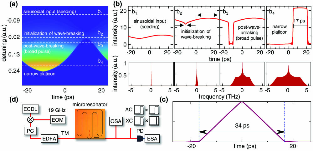
    Fig. 1. Platicon pulse generation in normal-dispersion frequency combs: operating regimes, numerical modeling, and modulated pump experimental setup. (a) 2D evolution map of platicon temporal profile as a function of intracavity fast time and detuning. Four characteristic stages are selected to show the details of the evolution in panel (b). (b) Upper panels: temporal profiles of the platicon at different evolution stages; lower panels: frequency spectra corresponding to each state. (b1) Sinusoidal input (seeding); (b2) initialization of wave breaking. Self-steepening shows that wave breaking is about to happen, with modulation maxima directed outwardly and minima directed inwardly. (b3) Post-wave breaking. Wave breaking happens, and a broad square pulse is generated; (b4) a shorter narrow platicon is generated for increasing red detuning, such as at δ=+0.2531. (c) The simulated autocorrelation of the square pulse shown in (b4). The width of the triangle is twice of the width of the square pulse. (d) Schematic setup of platicon generation. The cw laser from the ECDL is first modulated by an EOM, and the modulation frequency is chosen to match the single FSR (19.547  GHz). After amplification by an EDFA, the modulated pump is launched into the single-mode microresonator, and the pump frequency is slowly red-tuned to generate the platicon. A polarization controller (PC) and a polarized beam splitter (not shown in the diagram) are utilized to optimize the intensity of TM polarization for TM mode operation. A 20 GHz high-speed photodetector (PD) is used to measure the amplitude and phase noises. An OSA is used to map the platicon spectrum. Then the time-domain dynamics is examined by both autocorrelation (AC) and dual-comb cross correlation (XC). The actual single-mode microresonator is shown in the middle micrograph, whose straight waveguide is tapered from 2.5 to 1 μm to maintain high quality factor. The curved regions are 1 μm in width to maintain our single-mode frequency comb operation. Scale bar: 200 μm.
    Dynamic detuning evolution and spectra of a modulated-pump platicon frequency comb. (a) Pump transmission versus detuning. The comb evolves to its critical point at state 3 (blue). Left inset: optical spectra of states 1 (red) and 4 (black), in which there are only modulated pump spectra. The first pair of sidebands are about 3 dB in intensity lower than main pump. Right inset: FSR measurement of the microresonator. The fitted GVD is positive at 55 fs2/mm, and the fitted TOD is negative at −948 fs3/mm. (b) Comb spectra at states 2 and 3. The comb just starts to evolve due to spontaneous FWM at state 2 (green curve), and the spectrum shape is more like a triangle other than the frequency spectrum of a platicon. At state 3, the frequency comb spectrum (blue curve) is at the critical point, spanning 80 nm. The shape coincides with the simulation, shown in the upper left inset. The upper right inset is comb spectrum simulation with positive TOD as a comparison. A typical single-soliton comb spectrum envelope is included in the dashed pink line, indicating that the platicon has higher comb line power at wavelengths away from the pump.
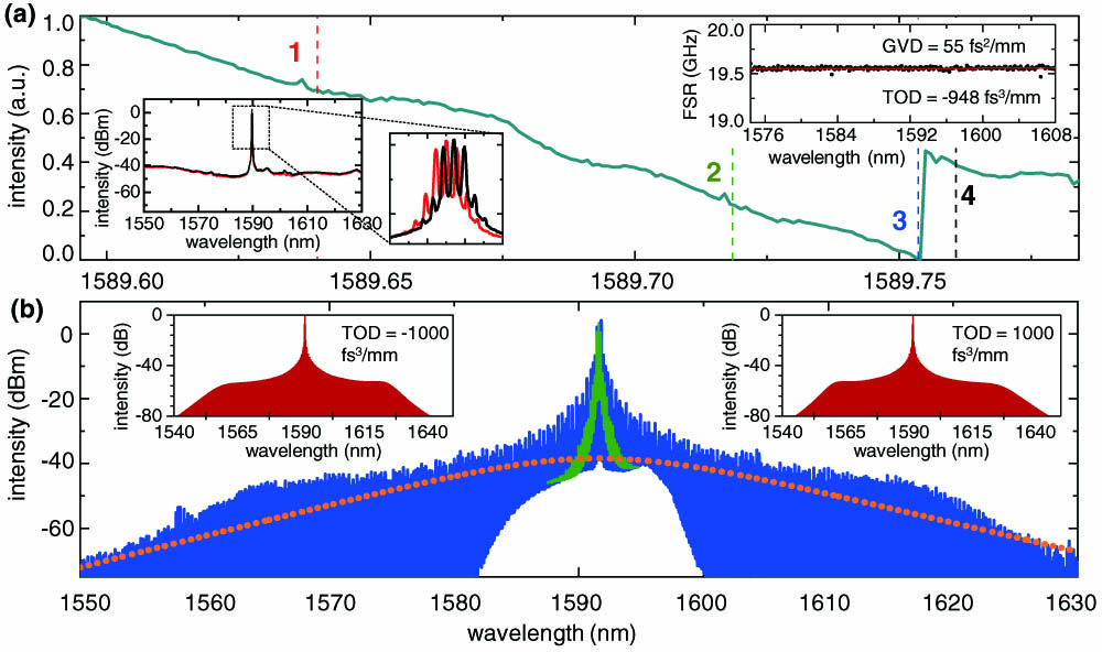
    Fig. 2. Dynamic detuning evolution and spectra of a modulated-pump platicon frequency comb. (a) Pump transmission versus detuning. The comb evolves to its critical point at state 3 (blue). Left inset: optical spectra of states 1 (red) and 4 (black), in which there are only modulated pump spectra. The first pair of sidebands are about 3 dB in intensity lower than main pump. Right inset: FSR measurement of the microresonator. The fitted GVD is positive at 55  fs2/mm, and the fitted TOD is negative at 948  fs3/mm. (b) Comb spectra at states 2 and 3. The comb just starts to evolve due to spontaneous FWM at state 2 (green curve), and the spectrum shape is more like a triangle other than the frequency spectrum of a platicon. At state 3, the frequency comb spectrum (blue curve) is at the critical point, spanning 80 nm. The shape coincides with the simulation, shown in the upper left inset. The upper right inset is comb spectrum simulation with positive TOD as a comparison. A typical single-soliton comb spectrum envelope is included in the dashed pink line, indicating that the platicon has higher comb line power at wavelengths away from the pump.
    Deterministic platicon comb formation controlled by the sideband modulation frequency. (a)–(c) Simulated frequency comb spectra with different modulation frequencies under a TOD of −1000 fs3/mm. (a) Δ=−1000 kHz, (b) Δ=0 kHz, (c) Δ=1000 kHz. (d)–(f) Experimental frequency comb spectra with different modulation frequencies. (d) 19.547 GHz (Δ≈−1000 kHz), (e) 19.548 GHz (Δ≈0 kHz), (f) 19.549 GHz (Δ≈1000 kHz). All comb spectra span around 80 nm. (g) Comb skewness versus sideband modulation frequency Δ. (h) Heterodyne beat note of the platicon frequency microcomb at different modulation frequency. The x axis is the offset frequency with respect to the FSR of pump mode. A 60 dB SNR is observed for each case. The RBW is 1 kHz. (i) Phase noise measurements of the LO and platicon comb. The phase noise of the platicon comb almost exactly follows the phase noise of the LO in the low-frequency range; except in the 1/f3 range, the platicon is slightly better. But starting from 1 MHz, the platicon comb outperforms the LO and suppresses the phase noise by up to 3 dB.
    Fig. 3. Deterministic platicon comb formation controlled by the sideband modulation frequency. (a)–(c) Simulated frequency comb spectra with different modulation frequencies under a TOD of 1000  fs3/mm. (a) Δ=1000  kHz, (b) Δ=0  kHz, (c) Δ=1000  kHz. (d)–(f) Experimental frequency comb spectra with different modulation frequencies. (d) 19.547 GHz (Δ1000  kHz), (e) 19.548 GHz (Δ0  kHz), (f) 19.549 GHz (Δ1000  kHz). All comb spectra span around 80 nm. (g) Comb skewness versus sideband modulation frequency Δ. (h) Heterodyne beat note of the platicon frequency microcomb at different modulation frequency. The x axis is the offset frequency with respect to the FSR of pump mode. A 60 dB SNR is observed for each case. The RBW is 1 kHz. (i) Phase noise measurements of the LO and platicon comb. The phase noise of the platicon comb almost exactly follows the phase noise of the LO in the low-frequency range; except in the 1/f3 range, the platicon is slightly better. But starting from 1 MHz, the platicon comb outperforms the LO and suppresses the phase noise by up to 3 dB.
    Pulse width characterization of platicon square pulses. (a) Schematic autocorrelation setup. BS, beam splitter; HWP, half-wave plate; APD, avalanche photodetector. (b) Schematic cross-correlation setup. PBS, polarized beam splitter. (c) Time-domain autocorrelation of the platicon comb. The bottom width of 34 ps of the triangle shape indicates a square bright pulse of 17 ps. (d) Cross correlation of the platicon pulse frequency comb. A 17 ps square bright pulse is directly observed. (e) Comb spectrum of a 4 ps platicon square pulse. The spacing between the two first minima is about 0.54 THz. The experimental measurement matches well with the simulation platicon comb spectrum (red curve). The inset is the time-domain square pulse simulation corresponding to the red curve, which proves a 4 ps square pulse generation. (f) Comb spectrum of a 2 ps platicon square pulse. The simulation of both the frequency and time domains shows a 2 ps square pulse generation. Left inset is the time-domain profile. Right inset is a summary of the platicon pulse widths versus δ, which indicates that narrow pulse width down to hundreds of femtoseconds could be achieved.
    Fig. 4. Pulse width characterization of platicon square pulses. (a) Schematic autocorrelation setup. BS, beam splitter; HWP, half-wave plate; APD, avalanche photodetector. (b) Schematic cross-correlation setup. PBS, polarized beam splitter. (c) Time-domain autocorrelation of the platicon comb. The bottom width of 34 ps of the triangle shape indicates a square bright pulse of 17 ps. (d) Cross correlation of the platicon pulse frequency comb. A 17 ps square bright pulse is directly observed. (e) Comb spectrum of a 4 ps platicon square pulse. The spacing between the two first minima is about 0.54 THz. The experimental measurement matches well with the simulation platicon comb spectrum (red curve). The inset is the time-domain square pulse simulation corresponding to the red curve, which proves a 4 ps square pulse generation. (f) Comb spectrum of a 2 ps platicon square pulse. The simulation of both the frequency and time domains shows a 2 ps square pulse generation. Left inset is the time-domain profile. Right inset is a summary of the platicon pulse widths versus δ, which indicates that narrow pulse width down to hundreds of femtoseconds could be achieved.
    Hao Liu, Shu-Wei Huang, Wenting Wang, Jinghui Yang, Mingbin Yu, Dim-Lee Kwong, Pierre Colman, Chee Wei Wong. Stimulated generation of deterministic platicon frequency microcombs[J]. Photonics Research, 2022, 10(8): 1877
    Download Citation