
A. Marcu, M. Stafe, M. Barbuta, R. Ungureanu, M. Serbanescu, B. Calin, N. Puscas. Photon energy transfer on titanium targets for laser thrusters[J]. High Power Laser Science and Engineering, 2022, 10(5): 05000e27
- High Power Laser Science and Engineering
- Vol. 10, Issue 5, 05000e27 (2022)
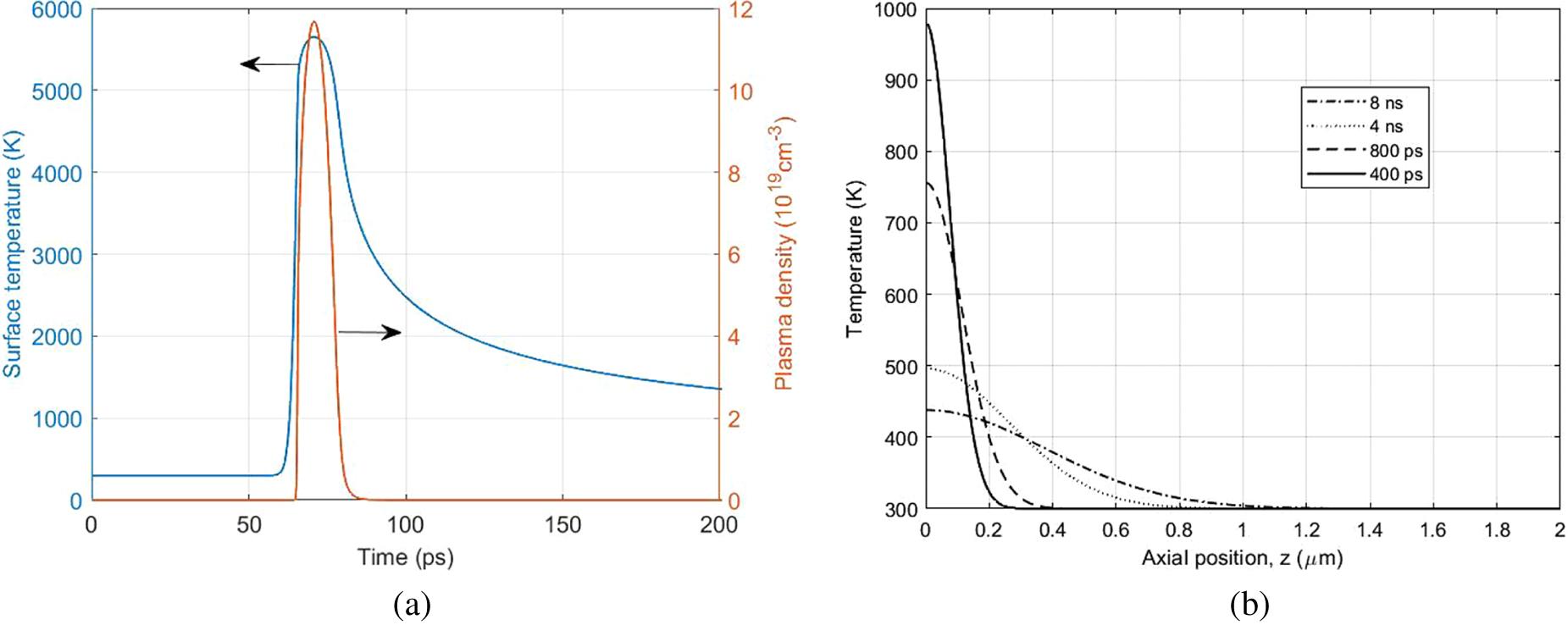
Fig. 1. Simulation results of (a) the time dependence of the surface temperature (left) and plasma density (right) and (b) the spatial profile along the axial direction at different moments after irradiation with a laser pulse with the following parameters: wavelength  = 800 nm, pulse duration
  = 7 ps and peak power density
  = 24 GW/cm2.
= 800 nm, pulse duration = 7 ps and peak power density = 24 GW/cm2. 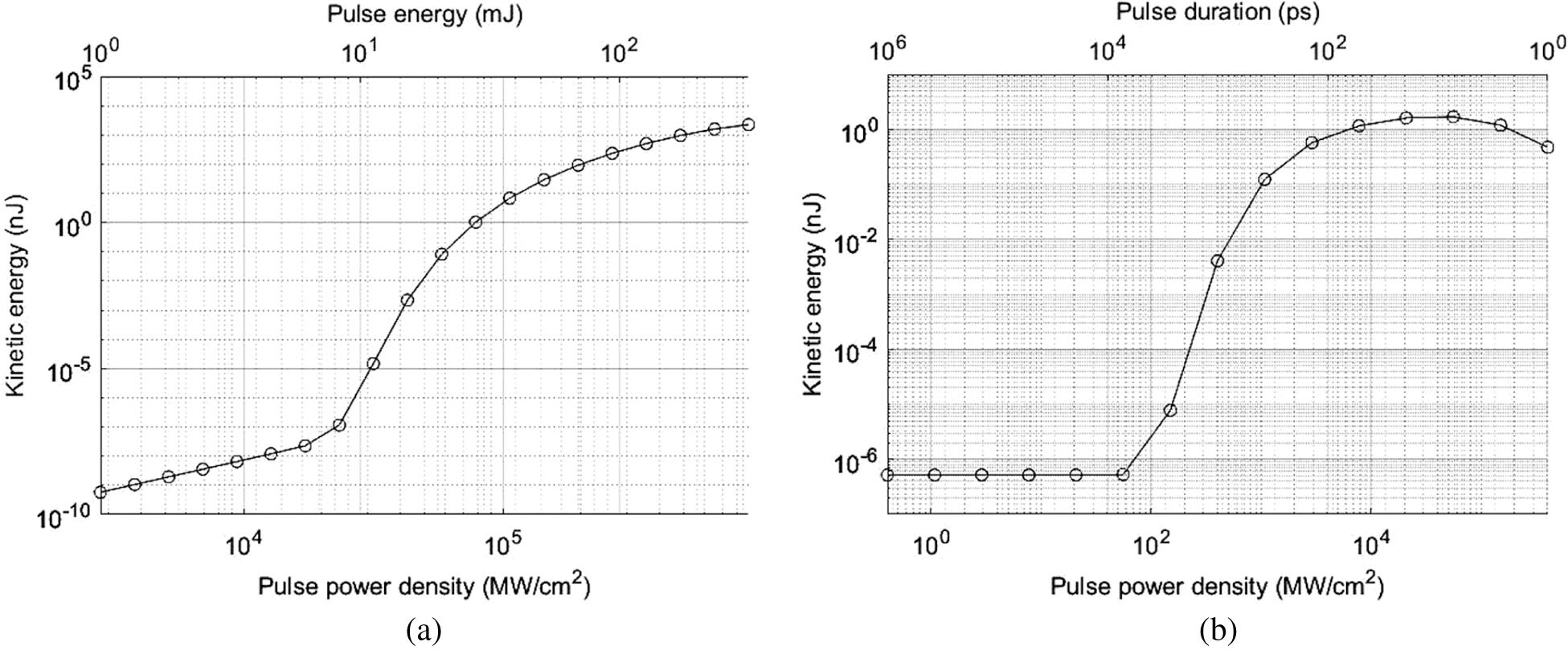
Fig. 2. Simulation results of kinetic energy  dependence on power density, controlled by: (a) pulse energy
  between 1 and 300 mJ,
  = 1064 nm,
  = 5.1 ps; (b) pulse duration
  between 1 ps and 1 μs for constant pulse energy
  = 30 mJ.
dependence on power density, controlled by: (a) pulse energy between 1 and 300 mJ, = 1064 nm, = 5.1 ps; (b) pulse duration between 1 ps and 1 μs for constant pulse energy = 30 mJ. Fig. 3. (a) Experimental setup of gravitational pendulum and (b) schematic forces diagram.
Fig. 4. Experimental results of kinetic energy transfer efficiency at different beam energies for (a) the multi-pulse ps laser (tuned train frequency from left to right in each series: 1000, 800, 625, 500 and 400 kHz) and (b) the single-pulse fs laser (with tuned duration from left to right in each series: 5100, 4200, 3000, 2100, 1500, 900, 300 and 30 fs).
Fig. 5. Simulation results of kinetic energy transfer efficiency dependence on (a) pulse duration and (b) power density. Experimental data points with error bars of 800 nm laser pulses are represented as blue ( = 30 mJ) and red (
 = 70 mJ).
= 30 mJ) and red ( = 70 mJ). Fig. 6. Experimental results of kinetic energy transfer efficiency variation with pulse energy for (a)  fs pulse duration and (b) different pulse durations within the ps range. (c) Transfer efficiency slope variation at different laser power densities for the same pulse energy variations.
fs pulse duration and (b) different pulse durations within the ps range. (c) Transfer efficiency slope variation at different laser power densities for the same pulse energy variations. Fig. 7. Simulation results of transfer efficiency variation with (a) pulse energy and (b) pulse power density represented for different pulse durations,  = 1.2, 3 and 5.1 ps, for a constant pulse energy
  = 200 mJ; the experimental data from Figure 6(b) are included as (red) triangles (800 nm,
  = 1.2 ps), (black) circles (800 nm,
  = 3 ps) and (green) diamonds (800 nm,
  = 5.1 ps) error bars.
= 1.2, 3 and 5.1 ps, for a constant pulse energy = 200 mJ; the experimental data from Figure 6(b) are included as (red) triangles (800 nm, = 1.2 ps), (black) circles (800 nm, = 3 ps) and (green) diamonds (800 nm, = 5.1 ps) error bars. Fig. 8. Experimental data on kinetic energy transfer efficiency variation with the number of pulses of 7 ps and 1064 nm, at different laser frequencies, for comparable power densities.
Fig. 9. Experimental frequency influence on (1064 nm 7ps) laser impulse transfer for different average powers  : (a) 8.15 W; (b) 10.2 W; (c) 14.55 W.
: (a) 8.15 W; (b) 10.2 W; (c) 14.55 W. Fig. 10. (a) Simulation results of surface peak temperature versus pulse number. (b) Transfer efficiency versus pulse number. The blue curve and the inset plot correspond to ‘cooled’ targets down to 300 K before each consecutive pulse. (c) Transfer efficiency versus pulse number at three working frequencies.
Fig. 11. Simulation results of the transfer efficiency versus train duration: (a) by neglecting the heat accumulation between pulses and (b) by accounting for the heat accumulation between two consecutive pulses.
Fig. 12. (a) Experimental results of the power density influence on kinetic energy transfer efficiency for 20 ms trains of 7 ps pulses (1064 nm); inset, power density influence on slope variation. (b) Numerical results of the dependence of transfer efficiency on the pulse power density.
Fig. 13. Experimental results of kinetic energy transfer efficiency variation with power density for different train energies at (a) 20 ms, (b) 40 ms, (c) 80 ms and (d) 120 ms train duration.

Set citation alerts for the article
Please enter your email address
© Copyright 2018-2021 | Chinese Laser Press. All Rights Reserved 沪ICP备15018463号-20