
Xiao-Liang Li, Xian-Zhang Chen, Chen-Rong Liu, Liang Huang. Quantization condition of scarring states in complex soft-wall quantum billiards [J]. Acta Physica Sinica, 2020, 69(8): 080506-1
- Acta Physica Sinica
- Vol. 69, Issue 8, 080506-1 (2020)
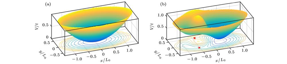
Fig. 1. (a) Two-dimensional harmonic potential (Eq. (2 )), where
 is the character scale of the system,
 , and
, and
 . To break the discrete symmetry, we added a
 potential at
 ; (b) On the potential given in Fig.(a), we added an additional Gaussian potential
 , where
 ,
,
 , and
, and
 . Thus the potential field forms two valleys and one peak, and the position of the bottom of the right valley is
 , with corresponding potential
 . There are two saddle points between the two valleys, as marked by the crosses, with corresponding potential values 0.591
t and 0.976t .
is the character scale of the system,
, and
. To break the discrete symmetry, we added a
potential at
; (b) On the potential given in Fig.(a), we added an additional Gaussian potential
, where
,
, and
. Thus the potential field forms two valleys and one peak, and the position of the bottom of the right valley is
, with corresponding potential
. There are two saddle points between the two valleys, as marked by the crosses, with corresponding potential values 0.591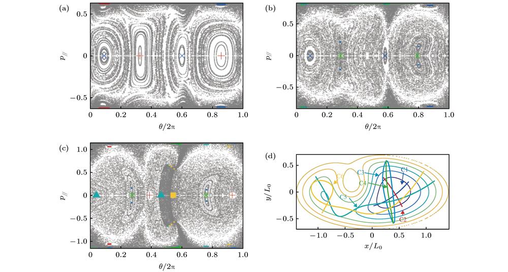
Fig. 2. The Poincaré section of the motion of a particle moving in the potential field given by Fig. 1(b) , e.g., when
 ,
,
 vs. the angle
 of this point with respect to the bottom of the right valley
 ((a)–(c)). The total energy of the particle is
 (a),
(a),
 (b), and
 (c), respectively. (d) The six classes periodic orbits that will be discussed later.
,
vs. the angle
of this point with respect to the bottom of the right valley
((a)–(c)). The total energy of the particle is
(a),
(b), and
(c), respectively. (d) The six classes periodic orbits that will be discussed later. Fig. 3. The representative eigen-wavefunctions of the billiard Fig. 1(a) . Shown are the the square of the modulus of wavefunctions that are condensed on the Lissajous orbits. The ratio of the frequency in
 and
and
 directions are: (a)–(c) 1∶2, (d) 2∶3, (e) 3∶4, (f) 1∶3. For all case,
 , the range of
 is
is
 and the value of the harmonic potential at the
 boundary is
 .
.
and
directions are: (a)–(c) 1∶2, (d) 2∶3, (e) 3∶4, (f) 1∶3. For all case,
, the range of
is
and the value of the harmonic potential at the
boundary is
. Fig. 4. The quantum numbers
 along the trajectory vs. energy for bouncing ball states in the harmonic potential with a small perturbation. Crosses are the numbers of wavelengthes counted from the wavefunctions minus one, circles are derived from the semiclassical formulas: (a) Horizontal bouncing ball orbits; (b) vertical bouncing ball orbits. Insets show the difference
 between these two methods.
along the trajectory vs. energy for bouncing ball states in the harmonic potential with a small perturbation. Crosses are the numbers of wavelengthes counted from the wavefunctions minus one, circles are derived from the semiclassical formulas: (a) Horizontal bouncing ball orbits; (b) vertical bouncing ball orbits. Insets show the difference
between these two methods. Fig. 5. The quantization condition for the four types of scars for the harmonic potential with a small perturbation. Crosses are the numbers of wavelengthes counted from the wavefunctions minus one, circles are the quantum numbers derived from the semiclassical formulas. Insets show the difference
 between these two methods.
between these two methods. Fig. 6. Two types of bouncing ball orbits in the potential shown in Fig. 1(b) and their projections on the zero energy surface. The potential function and its equipotential lines are also plotted. The first class of orbits (C1) corresponds to the center point of the two most significant KAM islands for
 ,
,
 and
and
 in
in Fig. 2 , and (C2) corresponds to the center points of the KAM islands for
 ,
,
 and
and
 in
in Fig. 2(a) .
,
and
in ,
and
in Fig. 7. The quantum numbers
 along the trajectory vs. energy for bouncing ball states in the modified harmonic potential shown in
 Fig. 1(b) for C1 orbits (a) and C2 orbits (b). Crosses are the numbers of wavelengthes counted from the wavefunctions minus one, circles are derived from the semiclassical formulas. In each panel, the upper set of points are for
 , and the lower set of points are for
 . For C2 orbits, only when energy is small there are
 states. Insets show the difference
 (solid circles, left coordinates) between these two methods, and
 obtained from
 (empty circles, right coordinates), where the horizontal dashed line is the
 obtained from fitting to the data, and the corresponding energies
 are
are
 and
and
 for C1 and C2 orbits, respectively.
along the trajectory vs. energy for bouncing ball states in the modified harmonic potential shown in , and the lower set of points are for
. For C2 orbits, only when energy is small there are
states. Insets show the difference
(solid circles, left coordinates) between these two methods, and
obtained from
(empty circles, right coordinates), where the horizontal dashed line is the
obtained from fitting to the data, and the corresponding energies
are
and
for C1 and C2 orbits, respectively. Fig. 8. The quantum numbers
 along the trajectory vs energy.
 for all cases. Crosses are the numbers of wavelengthes counted from the wavefunctions minus one, circles are derived from the semiclassical formulas. (a)–(d) correspond to C3-C6 orbits, with
 ,
,
 ,
,
 and
and
 , respectively. Insets show some typical scarring states and the corresponding classical orbits, and the difference
 between these two methods. Note that C3 orbits only appear for
 when C2 becomes unstable. C4 is the other unstable branch of C2, and becomes stable only for
 . C5 and C6 are orbits connecting the two potential valleys, only appear when higher energy is high enough.
along the trajectory vs energy.
for all cases. Crosses are the numbers of wavelengthes counted from the wavefunctions minus one, circles are derived from the semiclassical formulas. (a)–(d) correspond to C3-C6 orbits, with
,
,
and
, respectively. Insets show some typical scarring states and the corresponding classical orbits, and the difference
between these two methods. Note that C3 orbits only appear for
when C2 becomes unstable. C4 is the other unstable branch of C2, and becomes stable only for
. C5 and C6 are orbits connecting the two potential valleys, only appear when higher energy is high enough. 
Set citation alerts for the article
Please enter your email address
© Copyright 2018-2021 | Chinese Laser Press. All Rights Reserved 沪ICP备15018463号-20