Fast-forming focused spots through a multimode fiber based on an adaptive parallel coordinate algorithm

Zhe Yin; Guodong Liu; Fengdong Chen; Bingguo Liu

doi:10.3788/COL201513.071404

Abstract

We propose an adaptive parallel coordinate (APC) algorithm for quickly forming a series of focused spots at a multimode fiber (MMF) output by controlling the MMF input field with a spatial light modulator (SLM). Only passing over the SLM once, we can obtain SLM reflectance to form focused spots on different positions. Compared with the transmission matrix method, our APC does not require iterations and massive calculations. The APC does not require as much access device time as the adaptive sequential coordinate ascent (SCA) algorithm. The experiment results demonstrate that the time taken to form 100 spots with our APC is 1/54th the time with the SCA.

In recent years, the methods of shaping^[1–5] and imaging^[6–9] for light transmission through turbid media have been of widespread interest. Applying the shaping and imaging theories of turbid media to a multimode fiber (MMF) has promoted the development of MMF imaging methods. This line of research is of great significance to realize a single-fiber scanning microscope^[10,11], satisfying the requirements of being fiber-based^[12,13] and of miniaturization for modern microscopy. There are several methods^[14] that concern using a spatial light modulator (SLM) to form scanning focused spots on an arbitrary position at the MMF output. The first method is to measure the transmission matrix^[15,16] between the SLM sub-region complex reflectance and the MMF output field to form a desired intensity distribution at the MMF output. However, the transmission matrix method adopts Gerchberg–Saxton and Yang–Gu algorithms which need many iterations and a large number of computations. The second method is digital phase conjugation technology to form scanning focused spots at the MMF output^[17–19]. In order to form focused spots on different positions, a mechanical calibration objective lens must be moved. The third method is the objective function method^[14,20,21] which does not need the information of the transmission matrix. The objective function is maximized or minimized by an optimization algorithm to obtain an SLM pattern. The third method with the relatively simple calculation has become a popular research topic in this field^[22].

Mahalati proposed the adaptive sequential coordinate ascent (SCA) algorithm^[14], which forms one focused spot with a global optimum solution after passing over the SLM once and is faster than genetic algorithms. In order to form focused spots, it requires passing over the SLM the same number of times as the number of focused spots.

The MMF output field is greatly affected by fiber deformation^[23]. The formation time of a focused spot should be minimized to maintain the stability of the MMF propagation. We propose an adaptive parallel coordinate (APC) algorithm, establish the experimental setup, analyze the relationship between the input and output light field of the system, and derive the phase relations between the objective function and the SLM reflectance.

Sign up for Chinese Optics Letters TOC. Get the latest issue of Chinese Optics Letters delivered right to you！Sign up now

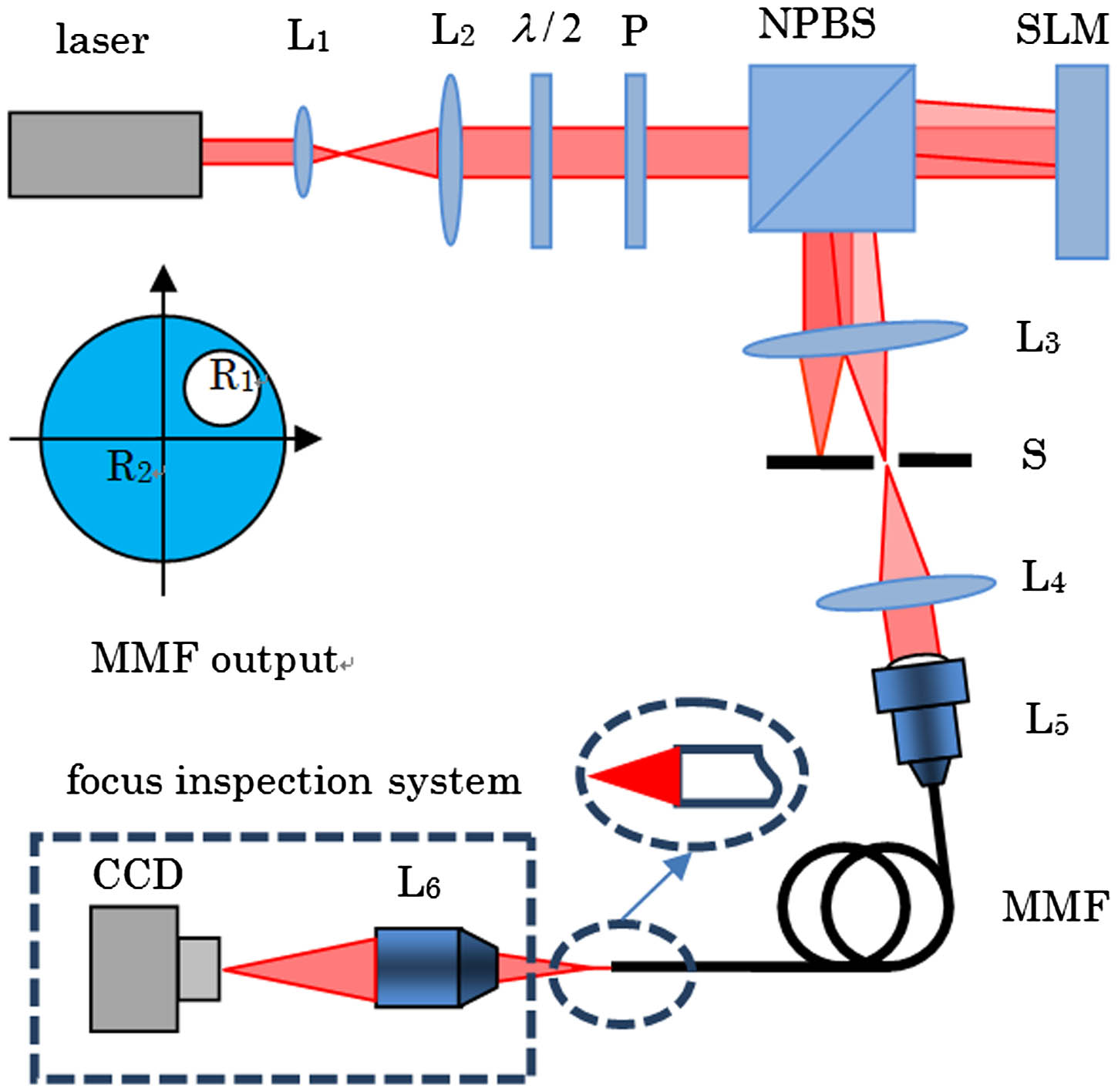
The experimental geometry is shown in Fig. 1. Linearly polarized light from a He–Ne laser is collimated and expanded to form parallel light by lenses $L_{1}$ and $L_{2}$ . The polarization direction of the beam is adjusted by a $λ / 2$ wave plate and the polarizer is consistent with the direction of the SLM optical axis. The light passes through a nonpolarizing beam splitter (NPBS) and is incident on the SLM. Loading the blaze grating phase on the SLM, the diffraction beam through the lens $L_{3}$ converges into several spots. Aperture S is used to block the beams except the first-order diffraction beam. The first-order diffraction beam is collimated by the lens $L_{4}$ , and coupled into the MMF by the fiber coupling lens $L_{5}$ . The plane on the distance 20 μm away from the MMF core at the MMF output is defined as the focal plane. The intensity distribution on the focal plane is magnified by a $20 \times$ objective lens $L_{6}$ and imaged on the CCD. In Fig. 1, inset, $R_{1}$ is the desired focused spot region, and $R_{2}$ is the outside of $R_{1}$ at the MMF output.

Figure 1.Experimental geometry for our APC algorithm.

We propose an APC algorithm to quickly form a series of desired focused spots at the MMF output with orthogonal modes decomposition theory^[24]. The light field on the SLM area can be divided into a series of square blocks which represent a series of orthogonal mode fields. Each block represents one mode which is orthogonal to each other. When all the modes meet at a point in space with the same phase, focused spots will be achieved.

The SLM is divided into $N$ sub-regions which represent a series of orthogonal modes. The first-order diffraction beam can pass the aperture and be coupled into the MMF, as shown in Fig. 1. The first-order diffraction beam is achieved by loading a blaze grating phase on the SLM sub-region. All the modes can be turned on or off independently by loading or not loading the blaze grating phase.

Our APC is divided into two processes. The first process is online recording. One fixed sub-region (considered to be covering the MMF output area) is selected as the reference mode which is gated with a blaze grating phase and keeps the phase unchanged. From the top-left corner of the SLM, a sub-region is selected as the test mode, gated with a blaze grating phase, and three different phases are loaded in succession. The fields of the reference mode and the test mode are interfered at the MMF output. The interference images are recorded by the CCD. Repeat the aforementioned operation to the next sub-region until all the sub-regions are finished. Then $3 N$ interference images are acquired. In Fig. 2, the white square regions represent an un-gated area. The stripe square regions represent the reference mode or the test mode. The black circle area represents a desired focused spot intensity distribution at the MMF output. The white spots represent focused spots.

Figure 2.Process of our APC algorithm.

The second process is offline APC computing. According to three interference images of the $k$ th test mode, optimization phases $p_{1}^{k}, p_{2}^{k}, \dots p_{M}^{k}$ of the $k$ th test mode for $M$ focused spots are acquired. Repeat the aforementioned operation for all the $N - 1$ test modes. The optimization phases of the $j$ th position are $p_{j}^{1}, p_{j}^{2}, \dots p_{j}^{N}$ . The reference mode is gated and loaded with zero phase. The other SLM sub-regions are gated simultaneously with loaded optimization phases. The focused spot will be formed.

To solve the optimization phase of our SLM, we analyze the relationship between the input and output light field of the system first. In Fig. 1, the SLM is placed on the Fourier plane of the MMF input. The equivalent focal length of the lenses $L_{3} - L_{4} - L_{5}$ is $f = f_{3} f_{5} / f_{4}$ . The light field at the MMF input $E_{SLM, out}$ is a Fourier transform of the SLM sub-region light field $E_{SLM, out}$ $E_{fiber, in} = L (E_{SLM, out}) = e^{i ϕ_{L}} E_{SLM, out},$ (1)where a linear operator $L$ is a Fourier transform, and $ϕ_{L}$ is the phase shift.

The reference mode and test mode are loaded simultaneously on the SLM. The SLM output field consists of the reference mode field $E_{SLM, ref} = A_{SLM, ref} e^{i ϕ_{SLM, ref}}$ and the test mode field $E_{SLM, test} = A_{SLM, test} e^{i ϕ_{SLM, test}}$ . The MMF input fields corresponding to the reference mode and the test mode are defined as follows $E_{fiber, in, ref} = L (E_{SLM, ref}) = A_{fiber, in, ref} e^{i (ϕ_{L} + ϕ_{SLM, ref})},$ (2) $E_{fiber, in, test} = L (E_{SLM, test}) = A_{fiber, in, test} e^{i (ϕ_{L} + ϕ_{SLM, test})},$ (3)where $A_{fiber, in, ref}$ and $A_{fiber, in, test}$ are the amplitude of $E_{fiber, in, ref}$ and $E_{fiber, in, test}$ , respectively.

We assume that the fiber is weakly guiding^[25,26], and ignore the loss of radiation modal energy and the changes of polarization state. The $M \times N$ complex matrix $P$ is the transmission matrix of the MMF. Term $u_{n}$ is the field at the MMF input and is described by $u_{n} = E_{fiber, in, ref} + E_{fiber, in, test} .$ (4)

According to the transmission matrix theory^[15], the field complex amplitude on the $m$ th position $(x, y)$ at the MMF output $v_{m}$ is $v_{m} = \sum_{n} P_{m n} u_{n} = \sum_{n} P_{m n} (E_{fiber, in, ref} + E_{fiber, in, test}) .$ (5)

Using Eqs. (2), (3), and (5) $v_{m} = \sum_{n} P_{m n} (A_{fiber, in, ref} e^{i (ϕ_{L} + ϕ_{SLM, ref})} + A_{fiber, in, test} e^{i (ϕ_{L} + ϕ_{SLM, test})}) = A_{ref} e^{i (ϕ_{L} + ϕ_{SLM, ref} + ϕ_{m, ref})} + A_{test} e^{i (ϕ_{L} + ϕ_{SLM, test} + ϕ_{m, test})},$ (6)where $P_{m, ref} = A_{m, ref} e^{i ϕ_{m, ref}}$ and $P_{m, test} = A_{m, test} e^{i ϕ_{m, test}}$ are the transmission parameters corresponding to the reference mode and the test mode, respectively. For simplicity of notation, we have defined $A_{ref} = A_{m, ref} A_{fiber, in, ref}$ and $A_{test} = A_{m, test} A_{fiber, in, test}$ .

Thus the MMF output intensity on the $m$ th position is described as $I_{fiber, out} (x, y) = {| A_{ref} |}^{2} + {| A_{test} |}^{2} + 2 | A_{ref} | | A_{test} | \cos [(ϕ_{SLM, ref} + ϕ_{m, ref}) - (ϕ_{SLM, test} + ϕ_{m, test})] = a (x, y) + b (x, y) \cos (ϕ_{SLM, test} - ϕ_{SLM, ref}) \cos δ (x, y) + b (x, y) \sin (ϕ_{SLM, test} - ϕ_{SLM, ref}) \sin δ (x, y),$ (7)where $δ (x, y) = ϕ_{m, ref} - ϕ_{m, test}$ , $a (x, y) = {| A_{ref} |}^{2} + {| A_{test} |}^{2}$ , and $b (x, y) = 2 | A_{ref} | | A_{test} |$ .

In Fig. 1, $R_{1}$ is defined as the desired focused spot region of the MMF output whose center is $(x_{m}, y_{m})$ . Term $R_{2}$ is defined as the region outside of $R_{1}$ at the MMF output. The total intensity at the MMF output is $I_{fiber, out, sum} = \iint_{R_{1} {+ R}_{2}} I_{fiber, out} (x, y) d x d y .$ (8)The normalized intensity on the $m$ th position $(x, y)$ at the MMF output is $I_{fiber, out, norm} = I_{fiber, out} (x, y) / I_{fiber, out, sum} .$ (9)The MMF output desired intensity profile is defined as a Gaussian profile $I_{des} (x, y) = I_{0} \exp [- a ({(x - x_{m})}^{2} + {(y - y_{m})}^{2})],$ (10)where $I_{0}$ is the normalized intensity, and $a$ is the parameter of the Gauss profile.

The objective function is defined as how close the actual MMF output intensity is to the desired MMF output intensity $F (ϕ_{SLM, test}) = \iint_{R_{1} {+ R}_{2}} | I_{des} - I_{fiber, out, norm} | d x d y = A + B \cos (ϕ_{SLM, test} - ϕ_{SLM, ref}) + C \sin (ϕ_{SLM, test} - ϕ_{SLM, ref}),$ (11) $A = \iint_{R_{1}} I_{des} d x d y - \iint_{R_{2}} I_{des} d x d y + (\iint_{R_{2}} a (x, y) d x d y - \iint_{R_{1}} a (x, y) d x d y) / I_{fiber, out, sum}, B = 2 (\iint_{R_{2}} b (x, y) \cos δ (x, y) - \iint_{R_{1}} b (x, y) \cos δ (x, y) d x d y) / I_{fiber, out, sum}, C = 2 (\iint_{R_{2}} b (x, y) \sin δ (x, y) d x d y - \iint_{R_{1}} b (x, y) \sin δ (x, y) d x d y) / I_{fiber, out, sum} .$ (12)

We adopt the three-frame phase-stepping algorithm to obtain the optimal SLM reflectance. We set $ϕ_{SLM, ref} = 0$ . Three constant phases $ϕ_{SLM, test} = 0$ , $ϕ_{SLM, test} = 2 π / 3$ , and $ϕ_{SLM, test} = 4 π / 3$ are loaded on the test mode successively. The intensity distribution images acquired by the CCD are used to calculate objective function values $F (0)$ , $F (2 π / 3)$ , and $F (4 π / 3)$ . According to Eq. (11), $A$ , $B$ , and $C$ are solved. Defining $θ = \tan^{- 1} (C / B)$ , the optimum phase of the test mode is $φ_{test, opt} = {\begin{cases} θ & if B \cos θ + C \sin θ < 0 \\ θ + π & otherwise \end{cases} .$ (13)

The experimental apparatus is shown in Fig. 3. The main instruments and devices are as follows: a 632.8 nm linear polarization He–Ne laser (Thorlabs 25-LHP-151-230), SLM (BNS P512–635, $512 pixels \times 512 pixels$ , pixel size is $15 μm \times 15 μm$ ), doublet lens $L_{3}$ ( $f = 150 mm$ ), doublet lens $L_{4}$ ( $f = 125 mm$ ), doublet lens $L_{5}$ (Thorlabs F810SMA-635 $f = 35.4 mm$ ), MMF (Thorlabs M14L01, the core diameter is 50 μm, the length is 1 m, and $NA = 0.19$ ), CCD (AVT F145B), and the microscope $L_{6}$ (Moritex $20 \times$ ). There is no vibration source around the experimental platform. We adopt a damping layer to reduce the vibration.

Figure 3.Experimental apparatus.

As shown in Fig. 4, $10 \times 10$ focused spots are formed with our APC at 100 completely different locations. Divide the SLM into $16 blocks \times 16 blocks$ to obtain 256 sub-regions. Online recording time is 180 s. Offline computing time is 156 s. The total time is 336 s. Some spots cannot be formed because the MMF output beam profile is a circle where some of the focused spots are outside of the circle.

Figure 4.One hundred focused spots with our APC.

The focused efficiency of a focused spot is defined as the ratio of the intensity in the focused spot area to the total MMF output intensity. Figure 5 shows 100 focused spot efficiencies under different reference modes with APC. Excluding the spots which cannot be formed, the average focused efficiency is 9.2%, 7.5%, and 6% under the reference mode separately located in the center block (8,8), the top block (3,8), and the left block (8,3) of the SLM ( $16 \times 16$ ). The maximal focused efficiency is 17.5%, 14.1%, and 12.4%, respectively, under three reference modes. The reference mode is a sub-region of the SLM. There is a small amount of the light beam that is coupled into the MMF for the reference mode at the edge of SLM. At the MMF output, the reference mode beam is too weak to be detected completely by the CCD. The intensity of reference mode (8,8) is 3 times the intensity of reference mode (3,8) and 8 times the intensity of reference mode (8,3). The reference mode located at the center of the SLM exhibits higher average focused efficiencies than the reference mode located at the edge of the SLM.

Figure 5.Focused efficiency of 100 spots with our APC.

Forming a focused spot at the center of the MMF output after 2500 steps with Monte Carlo^[20,21], the focused efficiency is 14%, which is lower than the efficiency with our APC. The focused efficiency of the focused spot located in the center of the MMF output with the SCA is 22%, which is 1.3 times the focused efficiency with our APC. In the SCA optimization process, the field controlled by the SLM is modified and optimized step by step. In the APC optimization process, one sub-region of the SLM is selected as the reference mode whose field distribution is un-changed. The APC may not obtain the global optimization SLM reflectance. So, the focused efficiency of focused spots with the SCA is better than with our APC.

The compared results in terms of the time taken between our APC and the SCA are shown in Table 1. $T_{APC}$ is the time taken by the APC algorithm. $T_{SCA}$ is the time taken by the SCA algorithm. Term ${ratio}_{T}$ is equal to $T_{APC} / T_{SCA}$ . If a parallel graphics card graphics processing unit (GPU) is adopted, ${ratio}_{T}$ can be much smaller.

Number of Focused Spots	TAPC (s)	TSCA (s)	RatioT
1	180	180	1
64	285	11,520	1/40
100	336	18,000	1/54

Table 1. Time Taken between the APC and SCA

View all Tables

In conclusion, we propose an APC algorithm to quickly form a serial of desired focused spots at the MMF output by controlling the MMF input field with the SLM. The proposed method consists of an online recording process and offline computing process. Only passing over the SLM once, we can obtain the SLM reflectance of forming focused spots on different positions by offline computation. The proposed method remarkably shortens the time of the device access and reduces the temporary influence on the MMF propagation stability. Compared with the transmission matrix method, our APC does not require iterations and a large number of computations. Compared with the SCA, our APC does not require as much device access time. The experimental results demonstrated that the time taken with our APC to form 100 focused spots is about 1/54th the time taken with the SCA. The speed of forming focused spots can be further improved by the adoption of a GPU, a high-speed SLM, and a high-speed CCD.

References

[1] S. Tripathi, R. Paxman, T. Bifano, K. C. Toussaint. Opt. Express, 20, 16067(2012).

[2] I. M. Vellekoop, A. P. Mosk. Opt. Commun., 281, 3071(2008).

[3] S. M. Popoff, G. Lerosey, R. Carminati, M. Fink, A. C. Boccara, S. Gigan. Phys. Rev. Lett., 104, 100601(2010).

[4] I. M. Vellekoop, A. P. Mosk. Opt. Lett., 32, 2309(2007).

[5] H. E. Holland, M. Pil. Controlling the propagation of light in disordered scattering media.

[6] D. Psaltis, I. N. Papadopoulos. Nature, 491, 197(2012).

[7] I. N. Papadopoulos, S. Farahi, C. Moser, D. Psaltis. Opt. Lett., 38, 2776(2013).

[8] F. Helmchen, W. Denk. Nat. Methods, 2, 932(2005).

[9] Y. Zhang, J. Shi, H. Li, G. Zeng. Chin. Opt. Lett., 12, 011102(2014).

[10] I. N. Papadopoulos, S. Farahi, C. Mouser, D. Psaltis. Proceedings of Optics in the Life Sciences Congress Technical Digest, BM4A.1(2013).

[11] I. N. Papadopoulos, S. Farahi, C. Mouser, D. Psaltis. Biomed. Opt. Express, 4, 260(2013).