
Tuo Liu, Suwan Sun, You Gao, Siyu Wang, Yongyuan Chu, Hairun Guo. Optical microcombs in whispering gallery mode crystalline resonators with dispersive intermode interactions[J]. Photonics Research, 2022, 10(12): 2866
- Photonics Research
- Vol. 10, Issue 12, 2866 (2022)
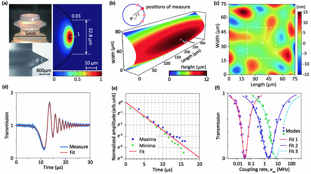
Fig. 1. Whispering gallery mode fluoride resonators. (a) Microscopic pictures of a home-made MgF 2 75 μm × 75 μm ± 15 nm 32.8 μm × 32.8 μm ± 5 nm MgF 2 Q 0 = 8.44 × 10 9 Q e = 1.1 × 10 10 Q Q = 4.75 × 10 9 e − 1 Q 4.95 × 10 9 MgF 2
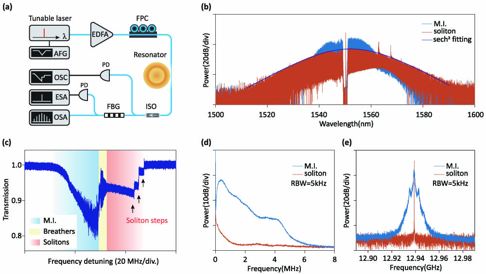
Fig. 2. Cavity Q > 60 dB O ( 10 kHz )
Fig. 3. Microcombs generated with the intermode pumping scheme. (a) Measured transmission of two resonances in proximity, probed by the laser at low power (ca. 3.8 mW). (b) The transmission of the same resonances probed at high power (ca. 281.7 mW), which reveals a soliton step. (c) Low noise RF spectrum of two combs [comb 1 and comb 2 shown in (d)] via the intermode pumping. (d) The measured comb spectra. Comb 1 is generated corresponding to the soliton step region in (b), while comb 2 is pumped regarding a second pair of resonances and is in a changed polarization state. Both combs feature intermode interactions on the central portion, and strong Raman lasing at both Stokes and anti-Stokes bands. In particular, a suspect anti-Stokes soliton comb is observed in comb 2. The full transmitted power is 238.2 mW (comb 1) and 197.3 mW (comb 2), respectively. The central comb power is estimated within the marked range (red arrows) such that the power of the Raman lasing is excluded in the calculation of power efficiency. Comb 3 is another observation that features broadband central power enhancement, and the overall spectral envelope is beyond the standard sech 2
Fig. 4. Simulated mode map of 20 transverse mode families in magnesium fluoride resonators. For each mode family (M.F.), the resonant frequencies are compared to a uniform frequency grid ω 0 + μ D 1 ω 0 / 2 π D 1 / 2 π
Fig. 5. Simulation of soliton combs with intermode interactions. (a)–(c) Dispersion profiles of two coupled mode families, in which the primary mode family (blue dots) is unchanged, and the auxiliary mode family (orange dots) shows three different profiles, corresponding to anomalous, normal, and close-to-zero dispersion with respect to the central mode (μ = 0 δ ω ( 1 − α ) | s out , p | 2 α | s out , aux | 2 | s out | 2
|
Table 1. Polishing Slurry Granule Size, Polishing Time, and Corresponding Roughness
| ||||||||||||||||||||||||||||||||||||||||||||||||||||||||||||||||||||||||||||||||
Table 2. Parameters for Numerical Simulations

Set citation alerts for the article
Please enter your email address
© Copyright 2018-2021 | Chinese Laser Press. All Rights Reserved 沪ICP备15018463号-20