Distinguishing node propagation influence by expected index of finite step propagation range

Xin Li; Cheng-Li Zhao; Yang-Yang Liu

doi:10.7498/aps.69.20191313

Journals >Acta Physica Sinica >Volume 69 >Issue 2 >Page 028901-1 > Article

Acta Physica Sinica
Vol. 69, Issue 2, 028901-1 (2020)

Distinguishing node propagation influence by expected index of finite step propagation range

Xin Li^*, Cheng-Li Zhao, and Yang-Yang Liu

DOI: 10.7498/aps.69.20191313 Cite this Article

Xin Li, Cheng-Li Zhao, Yang-Yang Liu. Distinguishing node propagation influence by expected index of finite step propagation range[J]. Acta Physica Sinica, 2020, 69(2): 028901-1 Copy Citation Text

show less

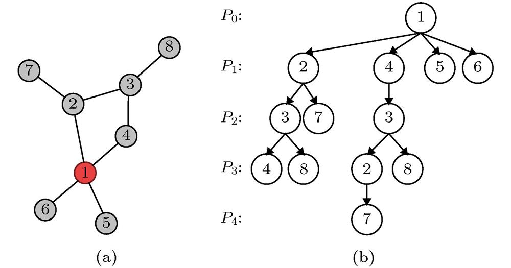
Fig. 1. A simple network example: (a) The network diagram; (b) the corresponding propagation tree of (a).一个简单网络例子　(a)网络图; (b)图(a)对应的传播树

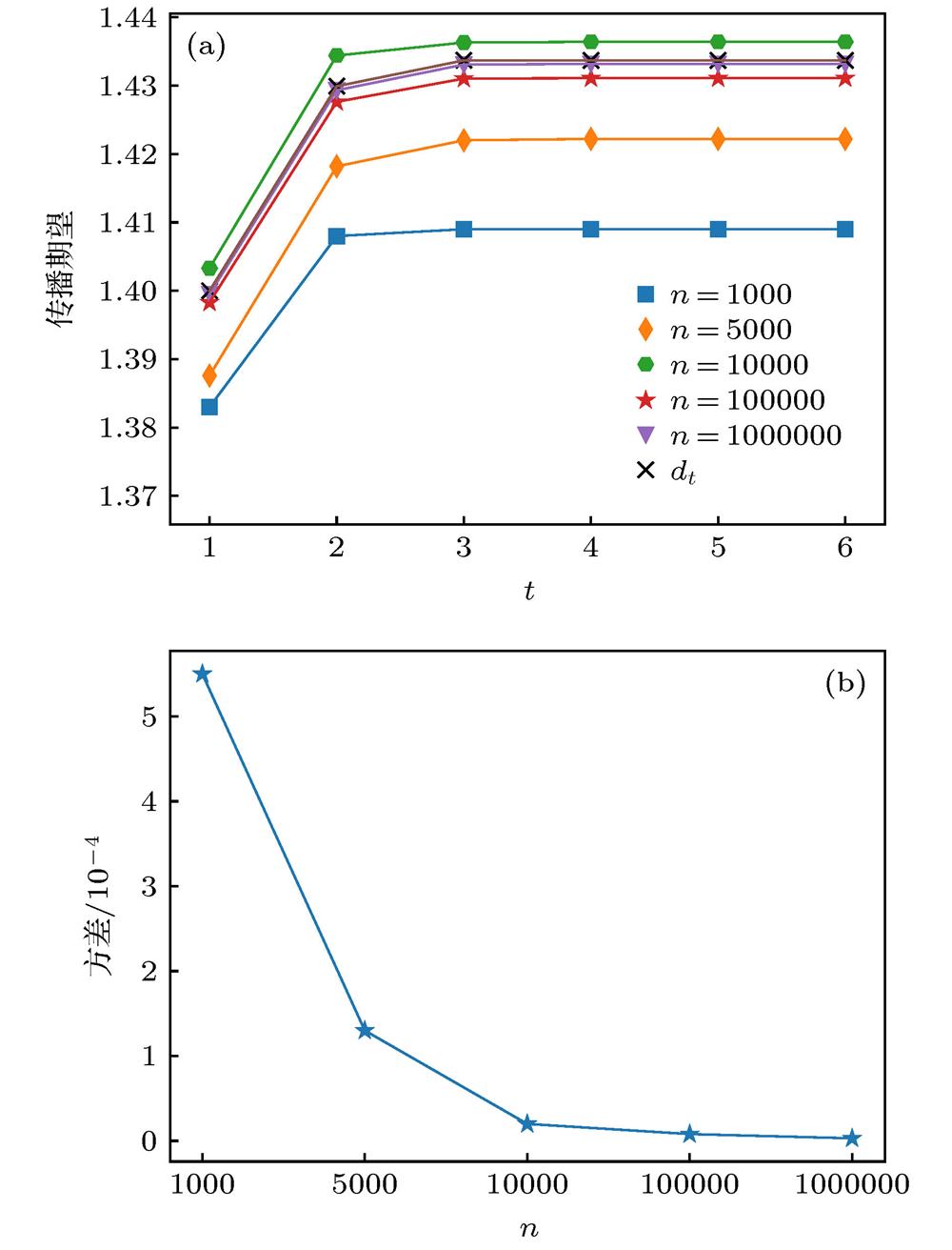
Download full size | View in the Article

(a) Approximate propagation expectation and the degree of propagation over time for different simulation times; (b) variance of the approximate propagation expectation and the degree of propagation of different simulation times.(a)不同仿真次数下的近似传播期望值和传播度随时间的变化; (b)不同仿真次数的近似传播期望值与传播度的方差变化

Fig. 2. (a) Approximate propagation expectation and the degree of propagation over time for different simulation times; (b) variance of the approximate propagation expectation and the degree of propagation of different simulation times.(a)不同仿真次数下的近似传播期望值和传播度随时间的变化; (b)不同仿真次数的近似传播期望值与传播度的方差变化

Download full size | View in the Article

Fig. 3. Changes of the 4th degree of propagation (normali-zed) of network node in Fig. 1 with the propagation pro-bability. 图1中的网络各节点4阶传播度(归一化)随传播概率变化

Download full size | View in the Article

Fig. 4. Flow chart of node influence maximization algorithm based on propagation degree.基于传播度的节点影响力极大化算法流程图

Download full size | View in the Article

Fig. 5. (a)−(c): Respectively reflects the relationship between the propagation capacity and degree, second-order propagation, and third-order propagation of several nodes randomly selected by the Deezer network, whereβ = 0.06; (d)−(f): Respectively reflects the global propagation probability of randomly selected nodes by the Deezer network (see reference[12]) Correspondence with degrees, second-order propagation, and third-order propagation, where β = 0.12 (here, it is not difficult to find through the simulation experiments that the percolation threshold of the network is between 0.06 and 0.12) (a)−(c) 分别反映了Deezer网络随机挑选若干节点的传播能力与度, 二阶传播度, 三阶传播度的关系, 其中β = 0.06; (d)−(f) 分别反映了Deezer网络随机挑选若干节点全局传播概率(参见文献[12])与度, 二阶传播度, 三阶传播度的对应情况, 其中β = 0.12(这里通过仿真实验不难发现该网络的渗流阈值介于0.06和0.12之间)

Download full size | View in the Article

Fig. 6. Kendall’s tau coefficient for different propagation probabilities, second-order, third-order propagation and simulation propagation ability.不同传播概率下度, 二阶、三阶传播度与仿真传播能力的kendall’s tau系数

Download full size | View in the Article

Fig. 7. (a) The relationship between the second-order propagation degree and the global propagation probability p in the case of the Email-Enron network with a propagation probability of 0.02; (b) the kendall's tau coefficient of each indicator with different propagation rates and propagation capabilities. (a)在Email-Enron网络中, 传播概率为0.02的情况下二阶传播度和全局传播概率p的关系; (b)各指标在不同概率下与传播能力的kendall’s tau系数

Download full size | View in the Article

Fig. 8. (a) The relationship between the second-order propagation degree and the global propagation probability p in the case of a Facebook network with a propagation probability of 0.09; (b) the kendall's tau coefficient of each indicator with different propagation rates and propagation capabilities. (a)在Facebook网络中, 传播概率为0.09的情况下二阶传播度和全局传播概率p的关系; (b)各指标在不同概率下与传播能力的kendall’s tau系数

Download full size | View in the Article

Fig. 9. In the Deezer network, (a) the variation of the propagation range with the number of selected seed nodes under different algorithms; (b) the variation of the global propagation probability with the number of seed nodes under different algorithms. The candidate nodes are 9792 nodes with a degree of 6, 7 and 8.在Deezer网络中(a)不同算法下传播范围随所选种子节点数量的变化和(b)不同算法下全局传播概率随种子节点数量的变化, 其中候选节点为度为6, 7, 8的9792个节点

Download full size | View in the Article

Fig. 10. (a), (b), and (c), (d), respectively, compare the propagation performance of Email-Enron, the selected seed node of the Facebook network under different algorithms.(a), (b)和(c), (d)分别比较了Email-Enron, Facebook网络在不同算法下所选种子节点的传播性能

Download full size | View in the Article

辅助算法二	联合概率算法
输入	时间t, 节点u以及对于u的序号集W
输出	联合概率 ${{{f}}_{{t}}}\left( {{{{u}}_{{W}}}} \right)$
1.	if W只含一个元素 then
2.	找到该节点的双亲节点 ${{{v}}_{\left( {{i}} \right)}}$
3.	${{{f}}_{{t}}}\left( {{{{u}}_{{W}}}} \right) = {{{f}}_{{{t}} - {{1}}}}\left( {{{{v}}_{\left( {{i}} \right)}}} \right) \times {{\beta }} \times \left( {{{1}} - {{{p}}_{{{t}} - {{1}}}}\left( {{u}} \right)} \right)$
4.	else
5.	找到传播树种 ${{{P}}_{{t}}}$代序号集为W的u节点, 记其双亲节点为 ${{{v}}_{{1}}}, {{{v}}_{{2}}}, \cdots , {{{v}}_{{l}}}$, 出现次数为 $ m_1, $$ m_2, \cdots , m_l$, 这些路径对于双亲节点的序号集分别为 ${{{X}}_{{1}}}, {{{X}}_{{2}}}, \cdots , {{{X}}_{{l}}}$, 对于节点u的序号集分别为 ${{{Y}}_{{1}}}, {{{Y}}_{{2}}}, \cdots {{{Y}}_{{l}}}$.
6.	for${{j}} = 0 \to {{l}}$do
7.	${{{f}}_{{t}}}\left( {{{{u}}_{{{{Y}}_{{j}}}}}} \right) = {{F}}\left( {{{t}} - {{1}}, {{{v}}_{{j}}}, {{{X}}_{{j}}}} \right) \times {{\beta }}$
8.	end for
9.	${{{f}}_{{t}}}\left( {{{{u}}_{{W}}}} \right) = \left[ {{{1}} - \mathop \prod \nolimits_{{{j}} = {{1}}}^{{l}} \left( {{{1}} - {{{f}}_{{t}}}\left( {{{{u}}_{{{{Y}}_{{j}}}}}} \right)} \right)} \right] \times \left( {{{1}} - {{{p}}_{{{t}} - {{1}}}}\left( {{u}} \right)} \right)$
10.	end if
11.	return${{{f}}_{{t}}}\left( {{{{u}}_{{W}}}} \right)$

Table 1.

Joint probability algorithm

联合概率算法

递推算法	求种子节点s阶传播度
输入	seed,${{\beta }}$, s
输出	${{{d}}_{{s}}}$
1.	${\rm Tree }_{s} = {\rm FTree }(\rm seed)$ %获取节点 ${{seed}}$的s阶传播树
2.	赋初值 ${ { {p} }_{ {0} } }\left( { { {\rm seed} } } \right) = { { {f} }_{ {0} } }\left( { { {\rm seed} } } \right) = { {1} }$, 其他情况 ${{{p}}_{{t}}}\left( {{u}} \right) = {{{f}}_{{t}}}\left( {{u}} \right) = {{0}}$
3.	for${{t}} = {{1}} \to {{s}}$do
4.	for${{{u}}_{{y}}} \in {{{P}}_{{t}}}$do %遍历传播树中 ${{{P}}_{{t}}}$代的个体
5.	获得 ${{{u}}_{{y}}}$的双亲节点 ${{{v}}_{{x}}}$ %表示节点u所在传播树层中第x个u节点
6.	${{{f}}_{{t}}}\left( {{{{u}}_{{y}}}} \right) = {{{f}}_{{{t}} - {{1}}}}\left( {{{{v}}_{{x}}}} \right) \times {{\beta }} \times \left( {{{1}} - {{{p}}_{{{t}} - {{1}}}}\left( {{u}} \right)} \right)$
7.	end for
8.	for${{u}} \in {{{P}}_{{t}}}$do
9.	获得u的序号集W %指 ${{{P}}_{{t}}}$代节点u出现次序构成的集合
10.	计算联合概率 ${{{f}}_{{t}}}\left( {{u}} \right) = {{F}}\left( {{{t}}, {{u}}, {{W}}} \right)$
11.	end for
12.	for$u \in {\rm Tree}_{s}$do
13.	${{{p}}_{{t}}}\left( {{u}} \right) = {{{p}}_{{{t}} - 1}}\left( {{u}} \right) + {{{f}}_{{t}}}\left( {{u}} \right)$
14.	end for
15.	end for
16.	${ { {d} }_{ {s} } }\left( { { \rm{seed} } } \right) = \mathop \sum \nolimits_{ {u} } { { {p} }_{ {s} } }\left( { {u} } \right)$
17.	return${{{d}}_{{s}}}$

Table 2.

Pseudocode of the algorithm flow for s order progpagation of the seed node.

种子节点s阶传播度的算法流程伪代码

Xin Li, Cheng-Li Zhao, Yang-Yang Liu. Distinguishing node propagation influence by expected index of finite step propagation range[J]. Acta Physica Sinica, 2020, 69(2): 028901-1

Download Citation

Tools

Save the article for my favorites

Paper Information