Quantum-limited localization and resolution in three dimensions

Ben Wang; Liang Xu; Jun-chi Li; Lijian Zhang

doi:10.1364/PRJ.417613

Abstract

As a method to extract information from optical systems, imaging can be viewed as a parameter estimation problem. The fundamental precision in locating one emitter or estimating the separation between two incoherent emitters is bounded below by the multiparameter quantum Cramér-Rao bound (QCRB). Multiparameter QCRB gives an intrinsic bound in parameter estimation. We determine the ultimate potential of quantum-limited imaging for improving the resolution of a far-field, diffraction-limited optical field within the paraxial approximation. We show that the quantum Fisher information matrix (QFIm) in about one emitter’s position is independent on its true value. We calculate the QFIm of two unequal-brightness emitters’ relative positions and intensities; the results show that only when the relative intensity and centroids of two-point sources, including longitudinal and transverse directions, are known exactly, the separation in different directions can be estimated simultaneously with finite precision. Our results give the upper bounds on certain far-field imaging technology and will find wide use in applications from microscopy to astrometry.

1. INTRODUCTION

Locating an emitter and estimating different emitters’ relative positions precisely are key tasks in imaging problems. The question of two-point resolution was first discussed by Rayleigh [1,2]. Rayleigh’s criterion states that two-point sources are resolvable when the maximum of the illuminance produced by one point coincides with the first minimum of the illuminance produced by the other point. This criterion sets the limit of resolving power of optical systems [1]. Many methods have been developed to bypass this limit by converting resolving multi-emitter to locating single emitters. Deterministic super-resolution methods such as stimulated emission depletion microscopy [3], reversible saturable optical fluorescence transitions microscopy [4], and saturated structured illumination microscopy [5] utilize the fluorophores’ nonlinear response to excitation, which leads to individual emitting of emitters. Stochastic super-resolution methods such as stochastic optical reconstruction microscopy [6] and photo-activated localization microscopy [7] utilize the different temporal behavior of light sources, which emit light at separate times and thereby become resolvable in time. Therefore, localization of a single emitter is also an essential and fundamental issue in imaging problems.

Imaging is, as its heart, a multiparameter problem [8]. Targets’ localization and resolution can be viewed as parameter estimation problems. Positions of emitters are treated as parameters encoded in quantum states. The minimal error to estimate these parameters is bounded by the Cramér-Rao lower bound (CRLB). To quantify the precision, researchers utilize Fisher information (FI) associated with CRLB.

Inspired by classical and quantum parameter estimation theory [9 –22], Tsang and coworkers [23] reexamined Rayleigh’s criterion. If only intensity is measured in traditional imaging, the CRLB tends to infinite as the separation between two-point sources decreases, which is called the Rayleigh curse. However, when the phase information is also taken into account, two incoherent point sources can be resolved no matter how close the separation is, which has been demonstrated in experiments [24 –28]. If the centroid of the two emitters is also an unknown nuisance parameter, the precision to estimate the separation will decrease. Measuring the centroid precisely first can recover the lost precision due to misalignment between the measurement apparatus and the centroid [23,29]. Two-photon interference can be performed to estimate the centroid and separation at the same time [30]. Further developments in this emerging field have addressed the problem in estimating separation and centroid of two unequal brightness sources [31 –33], locating more than two emitters [34], and resolving the two emitters in 3D space [35 –39], with partial coherence [40 –42] and complete coherence [43]. In addition, with the development of the super-resolution microscopy techniques mentioned above, the method to improve precision of locating a single emitter is also important. Efforts along this line include designing optimal point spread functions (PSFs) [44,45] and the quantum-limited longitudinal localization of a single emitter [46].

Sign up for Photonics Research TOC. Get the latest issue of Photonics Research delivered right to you！Sign up now

In this work, we generalize the quantum-limited super-resolution theory to the localization of a single emitter with symmetric PSF and resolution of two unequal-brightness emitters in 3D space with arbitrary PSF. In the perspective of multiparameter estimation theory, we show that three Cartesian coordinates of a single emitter’s position [Fig. 1(a)] can be estimated in a single measurement scheme. For a two-emitter system, we consider the most general situation with five parameters, including relative intensity, centroids, and separations in transverse and longitudinal directions [see Fig. 1(b)]. We show that only two separations can be measured simultaneously to attain the quantum limit for the most general situation. In some special cases, centroids and separations can be estimated precisely at the same time. Localization and resolution in three dimensions are important in microscopy and astrometry. Our theoretical framework will be useful in these fields.

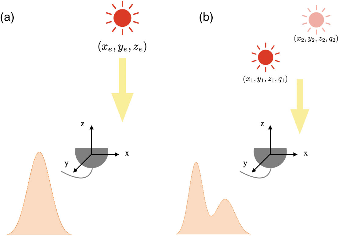
(a) Schematic of one emitter with position (x0,y0,z0). (b) Schematic of two emitters with positions (x1,y1,z1) and (x2,y2,z2) and different intensities (q1,q2).

Figure 1.(a) Schematic of one emitter with position ( $x_{0}, y_{0}, z_{0}$ ). (b) Schematic of two emitters with positions ( $x_{1}, y_{1}, z_{1}$ ) and ( $x_{2}, y_{2}, z_{2}$ ) and different intensities ( $q_{1}, q_{2}$ ).

Figure 2.Quantum and classical Fisher information of localization in 3D space. For estimation of the transverse coordinates of the emitter, the CFI coincides with the QFI in the position $z = 0$ , which indicates intensity measurement achieves QFI if the detector is put in the position of waist; for the estimation of the longitudinal coordinate, the detector needs to be put at the Rayleigh range to get the best precision.

This paper is organized as follows. In Section 2, we provide a quantum mechanical description of the optical system with one and two emitters; in Section 3, we will review the quantum estimation theory, the main method to quantify the precision of localization and resolution, and introduce the FI and quantum Fisher information (QFI). The specific expressions of QFI of localization and resolution with some discussions will be provided in Section 4, and analysis will be done on the results. Finally, we summarize all the results in Section 5.

2. QUANTUM DESCRIPTION OF LOCALIZATION AND RESOLUTION

We assume that the emitters are point-like sources and the electromagnetic wave emitted by the emitters is quasimonochromatic and paraxial, with ( $x$ , $y$ ) denoting the image-plane coordinates, $z$ denoting the distance from the emitters to the image plane. The quasimonochromatic paraxial wave $Ψ (x - x_{e}, y - y_{e}, z_{e})$ obeys the paraxial Helmholtz equation $\nabla_{T}^{2} Ψ + 2 k^{2} Ψ + i 2 k \frac{\partial}{\partial z} Ψ = 0,$ (1)where $(x_{e}, y_{e}, z_{e})$ are unknown coordinates of the emitter with respect to the coordinate origin defined in the image plane and $\nabla_{T}^{2} \equiv \partial^{2} / \partial x^{2} + \partial^{2} / \partial y^{2}$ . From Eq. (1), the generator of the displacement in direction $z$ is $\hat{G} = \frac{1}{2 k} \nabla_{T}^{2} + k$ . The generators of the displacement in direction $x$ and $y$ are momentum operators ${\hat{p}}_{x}$ and ${\hat{p}}_{y}$ , which are derivatives $- i \partial_{x}$ and $- i \partial_{y}$ . We have $Ψ (x - x_{e}, y - y_{e}, z_{e}) = \exp (- i \hat{G} z_{e} - i {\hat{p}}_{x} x_{e} - i {\hat{p}}_{y} y_{e}) Ψ (x, y,0)$ . Then, we rewrite the above results with quantum formulation and denote the PSF of the optical system $Ψ (x, y, 0) = ⟨ x, y | Ψ ⟩$ with $| x, y ⟩ = {\hat{a}}^{†} (x, y) | 0 ⟩$ . The quantum state of photons from a single emitter is $| \tilde{Ψ} ⟩ = \exp (- i \hat{G} z_{e} - i {\hat{p}}_{x} x_{e} - i {\hat{p}}_{y} y_{e}) | Ψ ⟩,$ (2)where $\tilde{Ψ}$ is the displaced wave function with respect to $Ψ (x, y,0)$ .

For two incoherent point sources, without the loss of generality, we only consider the displacement in the $x$ and $z$ directions. The quantum state is $ρ = q | Ψ_{1} ⟩ ⟨ Ψ_{1} | + (1 - q) | Ψ_{2} ⟩ ⟨ Ψ_{2} |,$ (3)where $| Ψ_{1,2} ⟩ = \exp (- i \hat{G} z_{1,2} - i {\hat{p}}_{x} x_{1,2}) | Ψ ⟩$ and $(x_{1}, z_{1}) (x_{2}, z_{2})$ are coordinates of two incoherent light sources. Here, the relative intensity $q$ is also an unknown parameter. The density matrix $ρ$ gives the normalized mean intensity $ρ (x) = q | Ψ (x - x_{1}, z_{1} {) |}^{2} + (1 - q) | Ψ (x - x_{2}, z_{2} {) |}^{2} .$ (4)Equations (3) and (4) can be reparameterized with the centroids $x_{0} \equiv (x_{1} + x_{2}) / 2$ , $z_{0} \equiv (z_{1} + z_{2}) / 2$ and separations $s \equiv x_{2} - x_{1}$ , $t \equiv z_{2} - z_{1}$ . The parameter vector is $θ \equiv {(x_{0}, d x, z_{0}, d z, q)}^{T}$ .

3. QUANTUM ESTIMATION THEORY

Localization and resolution can be treated as the estimation of the coordinates of emitters. In this section, we review the quantum and classical estimation theory for further analysis. The quantum states in localization and resolution problems are dependent on the parameters to be estimated. Let the parameters be $θ \equiv {θ_{1}, θ_{2}, θ_{3}, \dots}^{T}$ , and we use $θ_{i}$ to substitute the parameters in Eqs. (2) and (3) for convenience. A quantum measurement described by a positive operator-valued measure (POVM) $Π_{j}$ with the outcome $j$ is performed on the image plane to estimate $θ$ , so that the probability distribution of the outcome is $p (j | θ) = Tr [Π_{j} ρ (θ)]$ . The estimators are $θ̌ \equiv {{θ̌}_{1}, {θ̌}_{2}, {θ̌}_{3}, \dots}^{T}$ , which are the functions of measurement results. The precision of the estimates is quantified by the covariance matrix or mean square error $Cov [θ] \equiv \sum_{j} p (j | θ) [θ - θ̌ (j {)]}^{T} [θ - θ̌ (j)],$ (5)where $Cov [θ]$ is a positive symmetric matrix with a diagonal element denoting the variances of each estimator. The nondiagonal elements denote the covariance between different estimators.

For unbiased estimators, the covariance matrix is lower bounded by the Cramér-Rao bound $Cov [θ] \geq \frac{1}{M} {[F (ρ_{θ}, Π_{j})]}^{- 1},$ (6)where $M$ is the number of copies of the system to obtain the estimators $θ̌$ . $F (ρ_{θ}, Π_{j})$ is the Fisher information matrix (FIm) defined by ${[F (ρ_{θ}, Π_{j})]}_{μ ν} = \sum_{j} \frac{1}{p (j | θ)} \frac{\partial p (j | θ)}{\partial θ_{μ}} \frac{\partial p (j | θ)}{\partial θ_{ν}},$ (7)where $μ$ and $ν$ denote the row and column indices of the FIm. The inequality (6) means the matrix $Cov [θ] - \frac{1}{M} {[F (ρ_{θ}, Π_{j})]}^{- 1}$ is a semipositive definite matrix.

Here, we give an example of FIm that the measurement method is the intensity detection, projecting the quantum state into the eigenstates of the spatial coordinates. The elements of this POVM are ${Π_{x, y} = | x, y ⟩ ⟨ x, y |}$ , and the FIm $F_{μ ν}^{direct} = \iint \frac{1}{p (x, y | θ)} \frac{\partial p (x, y | θ)}{\partial θ_{μ}} \frac{\partial p (x, y | θ)}{\partial θ_{ν}} d x d y,$ (8)with $p (x, y) = Tr (ρ Π_{x, y})$ .

To obtain the ultimate precision, it is necessary to obtain the bound, which only depends on the quantum states rather than the measurement systems: $Cov [θ] \geq \frac{1}{M} {[F (ρ_{θ}, Π_{j})]}^{- 1} \geq \frac{1}{M} {[Q (ρ_{θ})]}^{- 1},$ (9)where the $Q (ρ_{θ})$ is the quantum Fisher information matrix (QFIm), which gives the maximum FIm. Its matrix elements are given by ${[Q (ρ_{θ})]}_{μ ν} = \frac{1}{2} Tr [ρ_{θ} {L_{μ}, L_{ν}}],$ (10)in which ${\cdot, \cdot}$ denotes the anticommutator, and $L_{κ}$ stands for the symmetric logarithmic derivative (SLD) with respect to the parameter $θ κ$ , which satisfies the condition $\partial_{κ} ρ_{θ} = \frac{L_{κ} ρ_{θ} + ρ_{θ} L_{κ}}{2} .$ (11)For the multiparameter estimation problem, an essential issue is the attainability of QCRB. If the system only has a single parameter to be estimated, the optimal measurement is to project the quantum state onto the eigenstates of the SLD [17], while this strategy is not suitable for multiple parameters. If the SLD operators $L_{κ}$ corresponding to the different parameters commute with each other $([L_{μ}, L_{ν}] = 0)$ , there exists a measurement that can maximize the parameters’ estimation precision simultaneously. If not, it does not imply this bound cannot be saturated. As discussed in Refs. [10,15,16], a sufficient and necessary condition for the saturability of the QCRB in inequality (9) is the satisfaction of a weak commutativity condition $Tr [ρ_{θ} {L_{μ}, L_{ν}}] = 0 .$ (12)We define the weak commutativity condition matrix $Γ (ρ_{θ})$ , and ${[Γ (ρ_{θ})]}_{μ ν} = \frac{1}{2 i} Tr [ρ_{θ} {L_{μ}, L_{ν}}]$ .

4. RESULTS

Our main results contain two parts. First, we show the QFIm of locating an emitter with symmetric wave functions satisfying the paraxial Helmholtz equation in 3D space. Second, we give the QFIm of two incoherent point sources in which the parameters to be estimated include relative intensity, centroids, and separations in both transverse and longitudinal directions.

A. Quantum Localization in 3D Space

In general, we assume that the wave function is symmetric in the transverse direction with respect to its center: $Ψ (x, y, z) = Ψ (- x, y, z) = Ψ (x, - y, z) .$ (13)Considering the situation of a single emitter, the quantum state is a pure state in Eq. (2). The SLD can be written in the simple expression $L_{κ} = 2 (| \tilde{Ψ} ⟩ ⟨ \partial_{κ} \tilde{Ψ} | + | \partial_{κ} \tilde{Ψ} ⟩ ⟨ \tilde{Ψ} |),$ (14)where $| \partial_{κ} \tilde{Ψ} ⟩ = \partial | \tilde{Ψ} ⟩ / \partial θ κ$ . Moreover, since $\partial_{κ} ⟨ \tilde{Ψ} | \tilde{Ψ} ⟩ = ⟨ \partial_{κ} \tilde{Ψ} | \tilde{Ψ} ⟩ + ⟨ \tilde{Ψ} | \partial_{κ} \tilde{Ψ} ⟩ = 0$ , the QFIm can be written in the form ${[Q_{loc} (θ)]}_{j k} = 4 Re (⟨ \partial_{j} \tilde{Ψ} | \partial_{k} \tilde{Ψ} ⟩ - ⟨ \partial_{j} \tilde{Ψ} | \tilde{Ψ} ⟩ ⟨ \tilde{Ψ} | \partial_{k} \tilde{Ψ} ⟩),$ (15)where Re denotes the real part. The specific forms of $| \partial_{κ} \tilde{Ψ} ⟩$ in this problem are $| \partial_{x_{e}} \tilde{Ψ} ⟩ = - i {\hat{p}}_{x} | \tilde{Ψ} ⟩, | \partial_{y_{e}} \tilde{Ψ} ⟩ = - i {\hat{p}}_{y} | \tilde{Ψ} ⟩, | \partial_{z_{e}} \tilde{Ψ} ⟩ = - i \hat{G} | \tilde{Ψ} ⟩,$ (16)because of the symmetry of the wave function in Eq. (13), $⟨ \tilde{Ψ} | \partial_{k} \tilde{Ψ} ⟩ = - ⟨ Ψ | \partial_{κ} | Ψ ⟩ = 0$ for any $κ = x, y$ . The weak commutativity condition is ${[Γ_{loc} (θ)]}_{j k} = 4 Im (⟨ \partial_{j} \tilde{Ψ} | \partial_{k} \tilde{Ψ} ⟩ - ⟨ \partial_{j} \tilde{Ψ} | \tilde{Ψ} ⟩ ⟨ \tilde{Ψ} | \partial_{k} \tilde{Ψ} ⟩),$ (17)where Im denotes the imaginary part. According to Eqs. (15) and (16), we obtain the QFIm $Q_{loc} = 4 [\begin{matrix} p_{x}^{2} & 0 & 0 \\ 0 & p_{y}^{2} & 0 \\ 0 & 0 & g_{z}^{2} - G_{z}^{2} \end{matrix}],$ (18)with $p_{x} = \sqrt{⟨ Ψ | {\hat{p}}_{x}^{2} | Ψ ⟩}$ , $p_{y} = \sqrt{⟨ Ψ | {\hat{p}}_{y}^{2} | Ψ ⟩}$ , $g_{z} = \sqrt{⟨ Ψ | {\hat{G}}^{2} | Ψ ⟩}$ , and $G_{z} = ⟨ Ψ | \hat{G} | Ψ ⟩$ . The weak commutativity condition is satisfied since $Γ_{loc} = [\begin{matrix} 0 & 0 & 0 \\ 0 & 0 & 0 \\ 0 & 0 & 0 \end{matrix}] .$ (19)This result indicates that the 3D localization problem is compatible [16], i.e., we can perform a single measurement to estimate all the parameters simultaneously and attain the precision achieved by optimal measurement for each parameter. If the generators for each parameter commute with each other $[{\hat{G}}_{i}, {\hat{G}}_{j}] = 0$ , the weak commutativity condition is always satisfied. This is indeed the situation for the generators ${\hat{p}}_{x}, {\hat{p}}_{y}$ and $\hat{G}$ .

We take the Gaussian beam as an example, which is the most common beam in practical experiments. The pure state without displacement in Eq. (2) is $| Ψ ⟩ = \int_{x, y} d x d y \sqrt{\frac{2}{π w_{0}^{2}}} \exp (- \frac{x^{2} + y^{2}}{w_{0}^{2}}) | x, y ⟩,$ (20)with $w_{0}$ the waist radius. The shifted wave function is $| \tilde{Ψ} ⟩ = \int_{x, y} d x d y \sqrt{\frac{2}{π w {(z_{e})}^{2}}} \exp [- \frac{{(x - x_{e})}^{2} + {(y - y_{e})}^{2}}{w {(z_{e})}^{2}}] \exp [- i k z_{e} - i k \frac{{(x - x_{e})}^{2} + {(y - y_{e})}^{2}}{2 R (z_{e})} + i ζ (z_{e})] | x, y ⟩,$ (21)with $w (z_{e}) = w_{0} \sqrt{1 + {(z_{e} / z_{r})}^{2}}$ , $R (z_{e}) = z_{e} [1 + {(z_{r} / z_{e})}^{2}]$ , and $ζ (z_{e}) = \tan^{- 1} (z_{e} / z_{r})$ , where $z_{r}$ is the Rayleigh range of a Gaussian beam, which equals $π w_{0}^{2} / λ$ related to the wavelength $λ$ .

The result of QFIm is $4 [\begin{matrix} \frac{1}{w_{0}^{2}} & 0 & 0 \\ 0 & \frac{1}{w_{0}^{2}} & 0 \\ 0 & 0 & \frac{1}{4 z_{r}^{2}} \end{matrix}] .$ (22)Considering the conventional intensity measurement, the classical Fisher information (CFI), according to Eq. (8), is $F_{μ ν} = \int_{x, y} d x d y \frac{1}{I (x, y)} \frac{\partial I (x, y)}{\partial θ_{μ}} \frac{\partial I (x, y)}{\partial θ_{ν}},$ (23)with $I (x, y) = | ⟨ x, y | \tilde{Ψ} ⟩ |^{2}$ , and the CFIs of three parameters are $F_{x_{e} x_{e}} = \frac{4 z_{r}^{2}}{w_{0}^{2} (z^{2} + z_{r}^{2})}, F_{y_{e} y_{e}} = \frac{4 z_{r}^{2}}{w_{0}^{2} (z^{2} + z_{r}^{2})}, F_{z_{e} z_{e}} = \frac{4 z^{2}}{{(z^{2} + z_{r}^{2})}^{2}} .$ (24)From these results, we can see that in Fig. 2, if only intensity measurement is applied when the detector is at the waist position, the CFIs for $x_{e}$ and $y_{e}$ equal the QFIs, while in the $z$ direction, the detector should be put at the Rayleigh range. Estimation of different parameters requires us to put the detector at different positions, which indicates that the intensity measurement is not the optimal measurement. The optimal measurement methods remain to be explored. To improve the precision of estimation, we can optimize the input state. Shaping the wave function to change the PSFs of optical systems is also helpful here [39,44,47]. The Laguerre–Gauss (LG) beam is also often used in experiments. Recent work shows that the precision to estimate the longitudinal position using an LG beam is better than using a Gaussian beam [48]. We also calculate the QFI of the transverse position of an LG beam and show the ratio between the QFI of a Gaussian beam and that of an LG beam in Table 1 with respect to the azimuthal mode index $p$ and radial index $l$ . The results show that using an LG beam to locate an emitter’s transverse position also has better performance than Gaussian.Table 1.

Ratio between the QFI of Gaussian Beam and That of LG Beam with Respect to the Azimuthal Mode Index $p$ and Radial Index $l$ ^a

${QFI}_{LG} / {QFI}_{G}$	$p = 0$	$p = 1$	$p = 2$	$p = 3$
$\| l \| = 0$	1	3	5	7
$\| l \| = 1$	2	4	6	8
$\| l \| = 2$	3	5	7	9
$\| l \| = 3$	4	6	8	10

Here, we select $p = 0, 1, 2, 3$ , and $l = 0, 1, 2, 3$ . $(p, l) = (0, 0)$ is the Gaussian beam.

B. Quantum Limited Resolution in Three Dimensions

Now we consider two incoherent point sources with the quantum state in Eq. (3). Different from single emitters, the quantum state is a mixed state, which implies that Eq. (15) cannot be used here. We need a new method to calculate the QFIm. According to the definition of SLD in Eq. (11), we find the quantum state $ρ$ and its derivatives, which is associated with SLDs supported in the subspace spanned by $| ψ_{1} ⟩$ , $| ψ_{2} ⟩$ , $\partial_{x_{1}} | ψ_{1} ⟩$ , $\partial_{z_{1}} | ψ_{1} ⟩$ , $\partial_{x_{2}} | ψ_{1} ⟩$ , and $\partial_{z_{2}} | ψ_{1} ⟩$ . Thus, similar to Ref. [38], our analysis relies on the expansion of the quantum state $ρ$ in the nonorthogonal but normalized basis: ${| Ψ_{1} ⟩, | Ψ_{2} ⟩, | Ψ_{3} ⟩, | Ψ_{4} ⟩, | Ψ_{5} ⟩, | Ψ_{6} ⟩},$ (25)where $| Ψ_{1} ⟩ = \exp (- i \hat{G} z_{1} - i \hat{p} x_{1}) | Ψ ⟩, | Ψ_{2} ⟩ = \exp (- i \hat{G} z_{2} - i \hat{p} x_{2}) | Ψ ⟩, | Ψ_{3} ⟩ = \frac{- i \hat{p} \exp (- i \hat{G} z_{1} - i \hat{p} x_{1}) | Ψ ⟩}{p}, | Ψ_{4} ⟩ = \frac{- i \hat{G} \exp (- i \hat{G} z_{1} - i \hat{p} x_{1}) | Ψ ⟩}{g}, | Ψ_{5} ⟩ = \frac{- i \hat{p} \exp (- i \hat{G} z_{2} - i \hat{p} x_{2}) | Ψ ⟩}{p}, | Ψ_{6} ⟩ = \frac{- i \hat{G} \exp (- i \hat{G} z_{2} - i \hat{p} x_{2}) | Ψ ⟩}{g},$ (26)with $p = \sqrt{⟨ Ψ | {\hat{p}}^{2} | Ψ ⟩}$ , $g = \sqrt{⟨ Ψ | {\hat{G}}^{2} | Ψ ⟩}$ . The relation between the representation of quantum states based on orthogonal basis and nonorthogonal basis is the linear transformation shown in Appendix A. The derivation of QFIm and the weak commutativity condition matrix is also shown in Appendix A. After a lengthy calculation, we obtain the two matrices: $Q = [\begin{matrix} Q_{x_{0} x_{0}} & 2 p^{2} (1 - 2 q) & Q_{x_{0} z_{0}} & 0 & 4 w \partial_{s} w \\ 2 p^{2} (1 - 2 q) & p^{2} & 0 & 0 & 0 \\ Q_{x_{0} z_{0}} & 0 & Q_{z_{0} z_{0}} & 2 (g^{2} - G^{2}) (- 1 + 2 q) & 4 w \partial_{t} w \\ 0 & 0 & 2 (g^{2} - G^{2}) (- 1 + 2 q) & g^{2} - G^{2} & 0 \\ 4 w \partial_{s} w & 0 & 4 w \partial_{t} w & 0 & \frac{- 1 + w^{2}}{(- 1 + q) q} \end{matrix}],$ (27) $Γ = [\begin{matrix} 0 & Γ_{x_{0} s} & Γ_{x_{0} z_{0}} & Γ_{x_{0} t} & 4 \partial_{s} ϕ (- 1 + 2 q) w^{2} \\ - Γ_{x_{0} s} & 0 & Γ_{s z_{0}} & 0 & - 2 \partial_{s} ϕ w^{2} \\ - Γ_{x_{0} z_{0}} & - Γ_{s z_{0}} & 0 & Γ_{z_{0} t} & 4 (G + \partial_{t} ϕ) (- 1 + 2 q) w^{2} \\ - Γ_{x_{0} t} & 0 & - Γ_{z_{0} t} & 0 & - 2 (G + \partial_{t} ϕ) w^{2} \\ - 4 \partial_{s} ϕ (- 1 + 2 q) w^{2} & 2 \partial_{s} ϕ w^{2} & - 4 (G + \partial_{t} ϕ) (- 1 + 2 q) w^{2} & 2 (G + \partial_{t} ϕ) w^{2} & 0 \end{matrix}],$ (28)where $w e^{i ϕ} = ⟨ Ψ_{1} | Ψ_{2} ⟩, G = ⟨ Ψ | \hat{G} | Ψ ⟩, Q_{x_{0} x_{0}} = 4 [p^{2} - 4 {(\partial_{s} w)}^{2} (1 - q) q - \frac{4 {(\partial_{s} ϕ)}^{2} (1 - q) q w^{2}}{1 - w^{2}}], Q_{x_{0} z_{0}} = 16 \partial_{s} w \partial_{t} w (- 1 + q) q - \frac{16 \partial_{s} ϕ (G + \partial_{t} ϕ) (- 1 + q) q w^{2}}{- 1 + w^{2}}, Q_{z_{0} z_{0}} = \frac{4 {G^{2} - 4 {(\partial_{t} w)}^{2} (- 1 + q) q - [G^{2} - 4 (G - \partial_{t} w + \partial_{t} ϕ) (G + \partial_{t} w + \partial_{t} ϕ) q (1 - q)] w^{2}}}{- 1 + w^{2}} + 4 g^{2}, Γ_{x_{0} s} = - \frac{8 \partial_{s} w \partial_{s} ϕ (- 1 + q) q w^{3}}{- 1 + w^{2}}, Γ_{x_{0} z_{0}} = - 16 [- \partial_{s} ϕ \partial_{t} w + \partial_{s} w (G + \partial_{t} ϕ)] (- 1 + q) q (- 1 + 2 q) w, Γ_{x_{0} t} = - \frac{8 (- 1 + q) q w [\partial_{s} ϕ \partial_{t} w + \partial_{s} w (G + \partial_{t} ϕ) (- 1 + w^{2})]}{- 1 + w^{2}}, Γ_{s z_{0}} = - \frac{8 (- 1 + q) q w [\partial_{s} w (G + \partial_{t} ϕ) + \partial_{s} ϕ \partial_{t} w (- 1 + w^{2})]}{- 1 + w^{2}}, Γ_{z_{0} t} = - \frac{8 \partial_{t} w (G + \partial_{t} ϕ) (- 1 + q) q w^{3}}{- 1 + w^{2}} .$ (29)If the separation in longitudinal direction is zero and the centroid in this direction is known, the matrix in Eq. (27) reduces to a $3 \times 3$ matrix, which is the same as the result in Ref. [31]. If the wave function satisfies the equation $G + \partial_{t} ϕ = 0,$ (30)the parameters $z_{0}$ , $t$ , and $q$ can be estimated with the precision given by QCRB simultaneously. In the most general case, for an arbitrary wave function, only the separations in $x$ and $z$ directions satisfy the weak commutativity condition. Therefore, the QFIm becomes $[\begin{matrix} p^{2} & 0 \\ 0 & g^{2} - G^{2} \end{matrix}],$ (31)in which each element is a constant. In brief, parameters on separations in $x$ and $z$ directions are compatible. In the multiparameter estimation problem, the achievable precision bound is the Helovo Cramér-Rao bound (HCRB) [49,50], denoted by $c_{h}$ . The discrepancy $D$ between QCRB and HCRB, which equals $c_{h} - Tr (Q^{- 1})$ is bounded by [51] $0 \leq D \leq Tr (Q^{- 1}) ℜ,$ (32)with $ℜ := {‖ i Γ Q^{- 1} ‖}_{\infty}$ , where ${‖ \cdot ‖}_{\infty}$ is the largest eigenvalue of a matrix. The first inequality is saturated if Eq. (12) is satisfied. $ℜ$ is a quantitative indicator of compatibility in multiparameter estimation problems whose value is between 0 and 1 [51]. Equation (32) shows that, if $ℜ$ equals zero, HCRB equals QCRB. Meanwhile, HCRB is at most twice QCRB [51,52].

We take the Gaussian beam in Eq. (21) as an example. We obtain $p = \frac{1}{w_{0}}$ , $g = \sqrt{k^{2} + \frac{2}{k^{2} w_{0}^{4}} - \frac{2}{w_{0}^{2}}}$ , $G = k - \frac{1}{k w_{0}^{2}}$ , $w = \sqrt{\frac{1}{1 + {(\frac{t}{2 z_{r}})}^{2}}} \exp (- \frac{k z_{r} s^{2}}{t^{2} + 4 z_{r}^{2}})$ , $ϕ = \arctan (\frac{t}{2 z_{r}}) - k t (1 + \frac{s^{2}}{2 t^{2} + 8 z_{r}^{2}})$ , and $g^{2} - G^{2} = 1 / k w_{0}^{4}$ . The condition in Eq. (30) is satisfied if $t = 0$ . Here, the value of $ℜ$ is shown in Fig. 3 with $w_{0} = 100 μm$ and wavelength $λ = 0.5 μm$ . In Fig. 3(a), the relative intensity is a constant $q = 0.5$ ; in the other three pictures, relative intensity is also a parameter to be estimated. From these results, we find $ℜ$ is close to zero in some regions, especially when the separations in two directions are nearly zero.

Figure 3.Contour plot of $ℜ$ of two Gaussian incoherent beams model in three dimensions in the ( $t$ , $s$ ) plane. (a) Relative intensity is a constant and equals to 0.5. (b) Relative intensity is also a parameter to be estimated; here, we set $q = 0.1$ . (c) Similar to (b) while $q = 0.3$ . (d) Similar to (b) while $q = 0.5$ .

When the separations in the $x$ and $z$ directions are infinitesimal (far less than the wavelength), the QFIm $Q_{G}$ and weak commutativity condition matrix $Γ_{G}$ of the Gaussian beam become $\lim_{s, t \to 0} Q_{G} = [\begin{matrix} \frac{2 k}{z_{r}} & \frac{k (1 - 2 q)}{z_{r}} & 0 & 0 & 0 \\ \frac{k (1 - 2 q)}{z_{r}} & \frac{k}{2 z_{r}} & 0 & 0 & 0 \\ 0 & 0 & \frac{1}{z_{r}^{2}} & \frac{- 1 + 2 q}{2 z_{r}^{2}} & 0 \\ 0 & 0 & \frac{- 1 + 2 q}{2 z_{r}^{2}} & \frac{1}{4 z_{r}^{2}} & 0 \\ 0 & 0 & 0 & 0 & 0 \end{matrix}],$ (33)and $\lim_{s, t \to 0} Γ_{G} = [\begin{matrix} 0 & 0 & 0 & 0 & 0 \\ 0 & 0 & 0 & 0 & 0 \\ 0 & 0 & 0 & 0 & 0 \\ 0 & 0 & 0 & 0 & 0 \\ 0 & 0 & 0 & 0 & 0 \end{matrix}],$ (34)indicating that, except the intensity, the other four parameters can be estimated simultaneously and the optimal precision of each parameter is a constant. Different intensities of the two emitters introduce the statistical correlations between the separation and centroid in the same direction. The parameters in different directions have negligible correlation, even though the intensities of two-point sources are different. Off-diagonal terms of QFIm lead to the inequality, ${[Q {(ρ_{θ})}^{- 1}]}_{j j} \geq 1 / Q {(ρ_{θ})}_{j j}$ , which means the existence of off-diagonal terms reduces the precision to estimate each parameter. Meanwhile, different intensities and the separation in the longitudinal direction arise the asymmetry of two-point sources, which reduces the precision to estimate the centroids in the transverse and longitudinal directions. Compared with Ref. [38], our results analyze how different intensities affect the four parameters in the transverse and longitudinal directions; here, relative intensity is also considered as an unknown parameter to be estimated. These results may find applications in subwavelength imaging.

5. CONCLUSION AND DISCUSSION

In summary, we give the general model and fundamental limitation for the localization of a single emitter and resolution of two emitters in 3D space. For one emitter, although the parameters in three directions are compatible with each other, the intensity detection cannot extract the maximal information of 3D positions simultaneously. Optimal measurement methods remain to be explored.

For two emitters, there are five parameters, including the relative intensity, separations, and centroids in the transverse and longitudinal directions of two emitters. We have obtained the quantum-limited resolution via the QFIm. In the most general case that one does not have any prior information of these parameters, only separations in the longitudinal and transverse directions can be estimated simultaneously to achieve the quantum-limited precision. More parameters can achieve the quantum-limited precision under special conditions, e.g., Eq. (30). The Gaussian beam example shows that, if and only if separation in longitudinal direction is zero, one can estimate separation, centroid in longitudinal direction, and the relative intensity with the quantum-limited precision. The example also shows that, when the separations in two directions are much smaller than the wavelength, all of the elements in the QFIm are constants, which indicates that separations and centroids in the longitudinal and transverse directions can be estimated precisely with a single measurement scheme. Spatial-mode demultiplexing [24 –26,53,54] or a mode sorter [35] can be useful here.

We should note that our results are suitable not only for Gaussian beams but also for arbitrary symmetric wave functions satisfying paraxial Helmholtz equations. Our results give a fundamental bound of quantum limit in localization and resolution in 3D space and will stimulate the development of new imaging methods.

APPENDIX A: SPECIFIC FORMULATIONS OF THE DERIVATIVE OF QUANTUM STATE

ρ | Ψ_{j} ? = q Π_{1 j} | Ψ_{1} ? + (1 ? q) Π_{2 j} | Ψ_{2} ?,

{[Q (ρ)]}_{μ ν} + i {[Γ (ρ)]}_{μ ν} = Tr [ρ L_{μ} L_{ν}],

References

[1] M. Born, E. Wolf. Principles of Optics, 461(1999).

[2] L. Rayleigh. XXXI. Investigations in optics, with special reference to the spectroscope. Philos. Mag., 8, 261-274(1879).

[3] S. W. Hell, J. Wichmann. Breaking the diffraction resolution limit by stimulated emission: stimulated-emission-depletion fluorescence microscopy. Opt. Lett., 19, 780-782(1994).

[4] R. Heintzmann, T. M. Jovin, C. Cremer. Saturated patterned excitation microscopy—a concept for optical resolution improvement. J. Opt. Soc. Am. A, 19, 1599-1609(2002).

[5] M. G. L. Gustafsson. Nonlinear structured-illumination microscopy: wide-field fluorescence imaging with theoretically unlimited resolution. Proc. Natl. Acad. Sci. USA, 102, 13081-13086(2005).

[6] M. J. Rust, M. Bates, X. Zhuang. Sub-diffraction-limit imaging by stochastic optical reconstruction microscopy (storm). Nat. Methods, 3, 793-796(2006).

[7] E. Betzig, G. H. Patterson, R. Sougrat, O. W. Lindwasser, S. Olenych, J. S. Bonifacino, M. W. Davidson, J. Lippincott-Schwartz, H. F. Hess. Imaging intracellular fluorescent proteins at nanometer resolution. Science, 313, 1642-1645(2006).

[8] L. A. Howard, G. G. Gillett, M. E. Pearce, R. A. Abrahao, T. J. Weinhold, P. Kok, A. G. White. Optimal imaging of remote bodies using quantum detectors. Phys. Rev. Lett., 123, 143604(2019).

[9] M. Szczykulska, T. Baumgratz, A. Datta. Multi-parameter quantum metrology. Adv. Phys. X, 1, 621-639(2016).

[10] K. Matsumoto. A new approach to the Cramér-Rao-type bound of the pure-state model. J. Phys. A, 35, 3111-3123(2002).

[11] L. Pezzè, M. A. Ciampini, N. Spagnolo, P. C. Humphreys, A. Datta, I. A. Walmsley, M. Barbieri, F. Sciarrino, A. Smerzi. Optimal measurements for simultaneous quantum estimation of multiple phases. Phys. Rev. Lett., 119, 130504(2017).

[12] O. Pinel, P. Jian, N. Treps, C. Fabre, D. Braun. Quantum parameter estimation using general single-mode Gaussian states. Phys. Rev. A, 88, 040102(2013).

[13] M. D. Vidrighin, G. Donati, M. G. Genoni, X.-M. Jin, W. S. Kolthammer, M. S. Kim, A. Datta, M. Barbieri, I. A. Walmsley. Joint estimation of phase and phase diffusion for quantum metrology. Nat. Commun., 5, 3532(2014).

[14] P. C. Humphreys, M. Barbieri, A. Datta, I. A. Walmsley. Quantum enhanced multiple phase estimation. Phys. Rev. Lett., 111, 070403(2013).

[15] P. J. D. Crowley, A. Datta, M. Barbieri, I. A. Walmsley. Tradeoff in simultaneous quantum-limited phase and loss estimation in interferometry. Phys. Rev. A, 89, 023845(2014).

[16] S. Ragy, M. Jarzyna, R. Demkowicz-Dobrzański. Compatibility in multiparameter quantum metrology. Phys. Rev. A, 94, 052108(2016).

[17] S. L. Braunstein, C. M. Caves. Statistical distance and the geometry of quantum states. Phys. Rev. Lett., 72, 3439-3443(1994).

[18] V. Giovannetti, S. Lloyd, L. Maccone. Advances in quantum metrology. Nat. Photonics, 5, 222-229(2011).

[19] V. Giovannetti, S. Lloyd, L. Maccone. Quantum metrology. Phys. Rev. Lett., 96, 010401(2006).

[20] J. Liu, H. Yuan, X.-M. Lu, X. Wang. Quantum fisher information matrix and multiparameter estimation. J. Phys. A, 53, 023001(2019).

[21] H. Yuan, C.-H. F. Fung. Quantum metrology matrix. Phys. Rev. A, 96, 012310(2017).

[22] Y. Chen, H. Yuan. Maximal quantum fisher information matrix. New J. Phys., 19, 063023(2017).

[23] M. Tsang, R. Nair, X.-M. Lu. Quantum theory of superresolution for two incoherent optical point sources. Phys. Rev. X, 6, 031033(2016).

[24] M. Paúr, B. Stoklasa, Z. Hradil, L. L. Sánchez-Soto, J. Rehacek. Achieving the ultimate optical resolution. Optica, 3, 1144-1147(2016).

[25] M. Tsang. Subdiffraction incoherent optical imaging via spatial-mode demultiplexing: Semiclassical treatment. Phys. Rev. A, 97, 023830(2018).

[26] M. Tsang. Subdiffraction incoherent optical imaging via spatial-mode demultiplexing. New J. Phys., 19, 023054(2017).

[27] W.-K. Tham, H. Ferretti, A. M. Steinberg. Beating Rayleigh’s curse by imaging using phase information. Phys. Rev. Lett., 118, 070801(2017).

[28] K. A. G. Bonsma-Fisher, W.-K. Tham, H. Ferretti, A. M. Steinberg. Realistic sub-Rayleigh imaging with phase-sensitive measurements. New J. Phys., 21, 093010(2019).

[29] M. R. Grace, Z. Dutton, A. Ashok, S. Guha. Approaching quantum limited super-resolution imaging without prior knowledge of the object location(2019).

[30] M. Parniak, S. Borówka, K. Boroszko, W. Wasilewski, K. Banaszek, R. Demkowicz-Dobrzański. Beating the Rayleigh limit using two-photon interference. Phys. Rev. Lett., 121, 250503(2018).

[31] J. Řehaček, Z. Hradil, B. Stoklasa, M. Paúr, J. Grover, A. Krzic, L. L. Sánchez-Soto. Multiparameter quantum metrology of incoherent point sources: towards realistic superresolution. Phys. Rev. A, 96, 062107(2017).

[32] J. Řeháček, Z. Hradil, D. Koutný, J. Grover, A. Krzic, L. L. Sánchez-Soto. Optimal measurements for quantum spatial superresolution. Phys. Rev. A, 98, 012103(2018).

[33] S. Prasad. Quantum limited super-resolution of an unequal-brightness source pair in three dimensions. Phys. Scr., 95, 054004(2020).

[34] E. Bisketzi, D. Branford, A. Datta. Quantum limits of localisation microscopy. New J. Phys., 21, 123032(2019).

[35] Y. Zhou, J. Yang, J. D. Hassett, S. M. H. Rafsanjani, M. Mirhosseini, A. N. Vamivakas, A. N. Jordan, Z. Shi, R. W. Boyd. Quantum-limited estimation of the axial separation of two incoherent point sources. Optica, 6, 534-541(2019).

[36] Z. Yu, S. Prasad. Quantum limited superresolution of an incoherent source pair in three dimensions. Phys. Rev. Lett., 121, 180504(2018).

[37] S. Prasad, Z. Yu. Quantum-limited superlocalization and superresolution of a source pair in three dimensions. Phys. Rev. A, 99, 022116(2019).

[38] C. Napoli, S. Piano, R. Leach, G. Adesso, T. Tufarelli. Towards superresolution surface metrology: quantum estimation of angular and axial separations. Phys. Rev. Lett., 122, 140505(2019).

[39] M. P. Backlund, Y. Shechtman, R. L. Walsworth. Fundamental precision bounds for three-dimensional optical localization microscopy with Poisson statistics. Phys. Rev. Lett., 121, 023904(2018).

[40] W. Larson, B. E. A. Saleh. Resurgence of Rayleigh’s curse in the presence of partial coherence. Optica, 5, 1382-1389(2018).

[41] M. Tsang, R. Nair. Resurgence of Rayleigh’s curse in the presence of partial coherence: comment. Optica, 6, 400-401(2019).

[42] W. Larson, B. E. A. Saleh. Resurgence of Rayleigh’s curse in the presence of partial coherence: reply. Optica, 6, 402-403(2019).

[43] Z. Hradil, J. Řeháček, L. Sánchez-Soto, B.-G. Englert. Quantum fisher information with coherence. Optica, 6, 1437-1440(2019).

[44] Y. Shechtman, S. J. Sahl, A. S. Backer, W. E. Moerner. Optimal point spread function design for 3D imaging. Phys. Rev. Lett., 113, 133902(2014).

[45] E. Nehme, B. Ferdman, L. E. Weiss, T. Naor, D. Freedman, T. Michaeli, Y. Shechtman. Learning an optimal PSF-pair for ultra-dense 3D localization microscopy(2020).

[46] J. Řeháček, M. Paúr, B. Stoklasa, D. Koutný, Z. Hradil, L. L. Sánchez-Soto. Intensity-based axial localization at the quantum limit. Phys. Rev. Lett., 123, 193601(2019).

[47] M. Paúr, B. Stoklasa, J. Grover, A. Krzic, L. L. Sánchez-Soto, Z. Hradil, J. Řeháček. Tempering Rayleigh’s curse with PSF shaping. Optica, 5, 1177-1180(2018).

[48] D. Koutný, Z. Hradil, J. Řeháček, L. L. Sánchez-Soto. Axial superlocalization with vortex beams. Quantum Sci. Technol., 6, 025021(2021).

[49] C. W. Helstrom, C. W. Helstrom. Quantum Detection and Estimation Theory, 3(1976).

[50] A. S. Holevo. Probabilistic and Statistical Aspects of Quantum Theory, 1(2011).

[51] A. Carollo, B. Spagnolo, A. A. Dubkov, D. Valenti. On quantumness in multi-parameter quantum estimation. J. Stat. Mech., 2019, 094010(2019).

[52] M. Tsang, F. Albarelli, A. Datta. Quantum semiparametric estimation. Phys. Rev. X, 10, 031023(2020).

[53] C. Datta, M. Jarzyna, Y. L. Len, K. Łukanowski, J. Kołodyński, K. Banaszek. Sub-Rayleigh resolution of incoherent sources by array homodyning(2020).

[54] Y. L. Len, C. Datta, M. Parniak, K. Banaszek. Resolution limits of spatial mode demultiplexing with noisy detection. Int. J. Quantum Inf., 18, 1941015(2020).

[55] L. J. Fiderer, T. Tufarelli, S. Piano, G. Adesso. General expressions for the quantum Fisher information matrix with applications to discrete quantum imaging(2020).