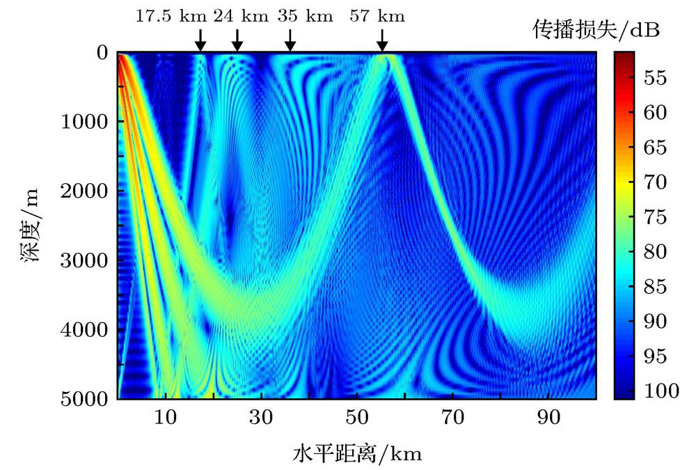
Fig. 1. Transmission loss variety with the change of distance and receiver depth in Munk sound channel.

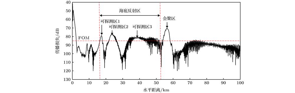
Fig. 2. Transmission loss variety with the change of distance in Munk sound channel when the receiver depth is fixed.

Fig. 3. Acoustic field distribution of angle dimension in Munk sound channel.

Fig. 4. Acoustic field formed by different normal mode (ray) clusters: (a) Acoustic field formed by normal mode 1 to normal mode 120 (rays with emanating angle from 0° to 9.5°); (b) acoustic field formed by normal mode 121 to normal mode 216 (rays with ema-nating angle from 9.5° to 18.2°); (c) acoustic field formed by normal mode 217 to normal mode 314 (rays with emanating angle from 18.2° to 27.6°); (d) acoustic field formed by normal mode 315 to norm al mode 354 (rays with emanating angle from 27.6° to 31.7°).

Fig. 5. Sketch map of two types of rays with the value of 20° in angle dimension.

Fig. 6. Comparison of WKBZ simulation and theoretical prediction about acoustic field distribution of angle dimension when source frequency varies (source depth is 50 m): (a) 100 Hz; (b) 200 Hz; (c) 300 Hz.

Fig. 7. Comparison of WKBZ simulation and theoretical prediction about acoustic field distribution of angle dimension when source depth varies (source frequency is 100 Hz): (a) 30 m; (b) 50 m; (c) 80 m.

Fig. 8. Comparison of WKBZ simulation and theoretical prediction about acoustic field distribution of angle dimension when sound velocity gradient varies: (a) Sound velocity profiles when sound velocity gradient varies; (b) comparison of results.

Fig. 9. Comparison of WKBZ simulation and theoretical prediction about acoustic field distribution of angle dimension when channel axis depth varies: (a) Sound velocity profiles when channel axis depth varies; (b) comparison of results.

Fig. 10. Comparison of WKBZ simulation and theoretical prediction about acoustic field distribution of angle dimension when sea depth varies: (a) Sound velocity profiles when sea depth varies; (b) comparison of results.

Fig. 11. Pulse signal design of active sonar based on acoustic field distribution of angle dimension.

Fig. 12. Acoustic field distribution of angle dimension.

Fig. 13. Array gain comparision between method of this article and the method of random setting: (a) Array gains of different methods; (b) transmission loss and distribution of detectable areas.