Effect of fabrication errors on multiple second-harmonic generation considering the pump depletion

Qiushuang Zhao; Liming Zhao

doi:10.3788/COL201513.S21901

Abstract

Second-harmonic generation (SHG) from aperiodic optical superlattices in the regime of pump depletion is investigated, when the influence of typical fabrication errors, which can be introduced by the random fluctuation of the thickness for each domain in the simulation, is considered in accordance with the actual case. It is found that both the SHG conversion efficiencies calculated in the undepleted pump approximation (UPA) and an exact solution decrease when the fluctuation increases; however, the decreasing degree is related to the wavelength of the fundamental wave (FW), and the longer the FW wavelength, the less the decrease in the corresponding conversion efficiency. A relative tolerance with respect to SHG conversion efficiency calculated in the UPA and exact solution is defined as previously [Opt. Express21, 17592 (2013)], in which a typical model based on the relative tolerance curves was proposed to estimate the SHG conversion efficiency. The simulation results show that the relative tolerance curves are basically coincident with the standard curve when the random fluctuation is very small (typically below 1%); however, as the fluctuation increases, the relative tolerance curves exhibit a large deviation from the standard curve, and the deviation is also determined by the wavelength of the FW.

Owing to access to the electric poling technique for domain inversion in ferroelectric crystals, quasi-phase-matching (QPM)^[1,2] has been extensively used in the context of various superlattices, including the periodic^[3,4], quasi-periodic^[5–7], nonperiodic^[8] optical superlattice, aperiodic optical superlattice (AOS)^[9–12], and disorder domain configuration^[13,14]. Note that all these structures aim at obtaining good phase matching and enhancing the optical frequency conversion, mostly focusing on second-harmonic generation (SHG). It is well-known that QPM is obtained under the undepleted pump approximation (UPA). However, when the conversion efficiency of SHG is high enough, the depletion of the fundamental wave (FW) cannot be ignored. Based on this case, more attention is focused on achieving compact and high-power laser pulses via SHG undergoing pump depletion^[15–20] into account. Recently, Zhao et al.^[18] report the applicability of multiple-QPM grating designed in UPA for SHG in the regime of pump depletion. The results show that the AOS sample devised in UPA applies to a general situation of low and high conversion efficiency of SHG, and a practical sample can be accurately evaluated by a developed model which can be shown by a relative tolerance curve, called the standard curve in this Letter. The relative tolerance is based on the SHG conversion efficiency calculated in the UPA and exact solution, which is only determined by the conversion efficiency with no relation to the pump intensity, preassigned wavelength, sample configuration, and the nonlinear media.

For the AOS configuration, samples are divided into layers^[21] arranged as alternating orientation of polarization, and the width of individual domain is optimized by simulated annealing (SA) algorithm. However, fabrication errors inevitably exist, and should be considered for an actual sample. Reference [18] gives the results for the perfect AOS sample; however, whether the conclusions proposed in Ref. [18] are still valid when the typical fabrication errors must be considered for realistic application. That is to say, how the random fluctuation impacts on the conversion efficiency of SHG in the UPA and exact solution; whether a relative tolerance curve will deviate from the standard curve is still in question. In this Letter, we will focus on investigating the aforementioned issues. This Letter starts with theoretical model for necessary formulas used in calculations, and the simulation results are presented with analyses. Finally, this paper concludes with a brief summary.

We first discuss a one-dimensional AOS sample made by ${LiNbO}_{3}$ (LN) crystal layers; the directions of polarization vectors in successive domains are opposite as are the signs of nonlinear optical coefficients. However, the width of each layer may be determined by the specified optical parametric processes. Each domain is parallel to the $y z$ -plane, and the propagation and the polarization directions of incident light are along the $x$ and $z$ axes, respectively. In the AOS sample, a FW $ω_{1} = ω$ is perpendicularly incident onto the surface, and the second harmonic wave (SHW) with $ω_{2} = 2 ω$ is generated by nonlinear optical process. In the assumption of slowing-wave variation of field amplitudes, the equations governing the propagation of the FW and the SHW are where $k_{1} = n_{1} ω / c$ ( $k_{2} = 2 n_{2} ω / c$ ), c is the light speed in vacuum, $n_{1} (n_{2})$ is the refractive index of the material at the FW (SHW) frequency, and $Δ k = k_{2} - 2 k_{1}$ denotes the wave vector mismatch between FW and SHW. In this context, we use $χ_{2} (x) = 2 | d_{33} | \tilde{d} (x),$ (2)where $\tilde{d} (x)$ (taking a binary value of 1 or $- 1$ ) represents the spatial distribution of the domain orientation. Since the field can be written in its real and imaginary parts $E_{α} (x) = ρ_{α} (x) e^{i ϕ_{α} (x)} (α = 1, 2)$ , the variable replacement is $u_{α} (x) = {(\frac{ε_{0} c^{2} k_{α}}{2 ω_{α} I})}^{1 / 2} ρ_{α} (x), α = 1, 2,$ (3)where $u_{α}^{2} (x)$ represents the normalized intensity, $L$ is the length of sample, and the conversion efficiency is given by $η = u_{2}^{2} (L) .$ (4)Via several substitutions and integrals as in Ref. [16], the exact solution $u_{2} (x_{n})$ can be obtained as long as the domain configuration is given. Consequently, the corresponding conversion efficiency will be achieved after the AOS sample is constructed.

Sign up for Chinese Optics Letters TOC. Get the latest issue of Chinese Optics Letters delivered right to you！Sign up now

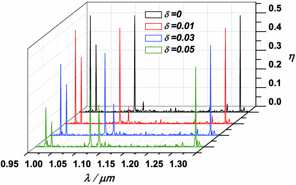
We adopt the following parameters in the designation of the AOS as: the pre-assigned FW wavelengths are $λ_{1} = 0.972 μm$ , $λ_{2} = 1.064 μm$ , and $λ_{3} = 1.283 μm$ . The number of domains $N = 1800$ , and the thickness of a single domain $Δ x = 3 μm$ . We set the intensity of the incident light waves as $I = 1.0 \times 10^{11} W / m^{2}$ , and $d_{33} = 27.0 pm / ν$ . An AOS sample which can achieve the aforementioned three wavelengths with high enough and nearly identical conversion efficiency of SHG is designed by the SA algorithm in the UPA. We impose a random distribution function $a a$ in the range of [0, 1] on the thickness of each block; therefore, the thickness of $i$ th block in a actual sample can be written as $d x (i) = Δ x + (a a - 0.5) / 0.5 * Δ x * δ$ in our simulation. Here $Δ x = 3 μm$ is the thickness of every block adopted in the perfect AOS sample. It can be deduced that $δ$ stands for the range of fabrication errors and $0 \leq δ \leq 1$ . For example, $δ = 0.01$ means $Δ x$ taking 1% random fluctuation around its accuracy, thus $\frac{d x (i) - Δ x}{Δ x}$ will be in the range of $[- 0.01, 0.01]$ . The conversion efficiency for the exact solution as a function of wavelength with different random fluctuations $δ$ is displayed in Fig. 1. The black curve is obtained from the devised AOS sample and the fabrication errors are not considered. While the fabrication errors are considered for the other curves, the red, blue, and green curves represent $δ = 0.01$ , 0.03, and 0.05, respectively. It is found that for the black curve, $η$ exhibits significant uniformity for the three preassigned wavelengths, except for two unexpected peaks with $λ = 0.984 μm$ and $λ = 1.082 μm$ appearing in the vicinity of $λ_{1}$ and $λ_{2}$ ; this denotes that the AOS sample can also achieve high and nearly coincident SHG conversion efficiency for an exact solution. For the other curves, the high conversion efficiency can also be achieved for the preset multiple wavelengths. However, the uniformity of the peak values is destroyed and the corresponding peak values decrease with the increase of $δ$ . For example, when $δ = 3 %$ , the $η$ for $λ_{1}$ reduces from 0.52 to 0.38, changing about 26%; for $λ_{3}$ , it varies from 0.52 to 0.48, decreasing about 6%. It is found that the longer wavelength suffers from less decrease for SHG conversion efficiency; this leads to the inconsistency of the peak values.

Figure 1.Variation of SHG conversion efficiency $η$ for an exact solution with the wavelength for different $δ$ . Black, red, blue, and green curves represent $δ = 0$ , 0.01, 0.03, and 0.05, respectively.

In order to further reveal the characteristic of the SHG in the constructed AOS with the consideration of fabrication errors, the variation of the exact solution with the sequence of domain for different random fluctuations $δ$ at the three wavelengths is presented in Fig. 2; Fig. 2(a) for $λ_{1} = 0.972 μm$ , Fig. 2(b) for $λ_{2} = 1.064 μm$ , and Fig. 2(c) for $λ_{3} = 1.283 μm$ ; the black, red, blue, orange, and green curves denote the case of $δ = 0$ , 0.01, 0.03, 0.05, and 0.07, respectively. For the black curve, $u_{2} (x_{n})$ is monotonically increasing with $n$ , which implies that the contribution of the individual block on the SHG process is positive, and good phase matching between FW and SHW can be achieved in the perfect AOS sample. However, when the random fluctuation is introduced and becomes increasingly large (especially beyond 3%), the variation of $u_{2} (x_{n})$ appears to be oscillating and the oscillation behavior grows more severe with the increase of $δ$ . For example, in Fig. 2(a), $u_{2} (x_{n})$ exhibits a dramatic decrease at the location of $n = 500$ , then begins to increase when $n = 800$ . The same case is shown for $λ = 1.064 μm$ , while for $λ = 1.283 μm$ , the oscillation is much weaker. These results obtained in our work indicate that the random fluctuation leads to the phase mismatch between the FW and SHW. Moreover, the phase mismatch is also related to wavelength, and the shorter wavelength, the stronger mismatch between the FW and SHW. This conclusion is also consistent with the fact obtained from Fig. 1 that the $η$ for $u_{2}$ shows less decrease for a longer wavelength with the same $δ$ .

Figure 2.Term $u_{2} (x_{n})$ versus the sequence of domain $n$ for the preassigned wavelengthes under different $δ$ : (a) 0.972, (b) 1.064, and (c) 1.283 μm. Black, red, blue, orange, and green curves represent $δ = 0$ , 0.01, 0.03, 0.05, and 0.07, respectively.

In Ref. [16], a relative tolerance is defined as $σ = \frac{{\tilde{u}}_{2} (x_{n}) - u_{2} (x_{n})}{u_{2} (x_{n})}$ to evaluate the difference of the SHG between the UPA and an exact solution. Term ${\tilde{u}}_{2} (x_{n})$ refers to the value calculated in the UPA. It is found that the relative tolerance is solely determined by the SHG conversion efficiency, but unrelated to the sample configuration, the nonlinear media, and the incident intensity. A model to assess $u_{2} (x_{n})$ was assumed as $σ = 0.0097 e^{u_{2} (x_{n}) / 0.217} (0.4 < u_{2} (x_{n}) < 0.9) .$ (5b)The model proves itself easy and convenient to estimate the SHG conversion efficiency when the pump depletion can not be ignored. However, Eq. (5) is fitted for the case of the perfect AOS configuration, and for an actual sample, fabrication errors are inevitably involved. We now proceed to discuss whether the developed model is fitted for the case when fabrication errors are introduced in an actual AOS sample. Figure 3 gives the variation of $σ$ versus $u_{2} (x_{n})$ under different $δ$ for $λ_{1} = 0.972 μm$ . The black curve represents the standard curve which can be obtained for Eq. (5), and the other red, blue, green, and orange curves stand for the cases of $δ = 0.01$ , 0.03, 0.05 and 0.07, respectively. It is clearly observed that the curves are inclined to deviate from the standard curve with the increase of $δ$ , except for $δ = 0.01$ , which is nearly coincident with the black curve. With the increase of $δ$ , there is a higher deviation. This is indicating that the deviation of a relative tolerance curve from the standard one is related to the FW wavelength. Figure 4 shows the relative tolerance curve for different FW wavelengths when $δ$ is set to 5%. The black curve is the standard curve, and the red, blue, and green curves successively correspond to $λ = 1.283$ , 1.064, and 0.972 μm. Clearly, for $λ = 0.972 μm$ , the relative tolerance curve appears serious deviation from the standard curve, while the departure degree is much smaller for $λ = 1.283 μm$ .

Figure 3.Variation of $σ$ as a function of $u_{2} (x_{n})$ for $λ = 0.972 μm$ . Black curve, standard curve according to Eq. (5); red, blue, green, and orange curves, data for $δ = 0.01$ , 0.03, 0.05, and 0.07, respectively.

Figure 4.Relative tolerance $σ$ with respect to $u_{2} (x_{n})$ for different FW wavelengthes under 5% random fluctuation. Red curve, data for $λ = 1.283 μm$ ; blue curve, data for $λ = 1.064 μm$ ; green curve, data for $λ = 0.972 μm$ ; black curve, standard curve in accordance with Eq. (5).

In conclusion, the conclusions obtained from Ref. [18] are redeveloped when the random fluctuation of the thickness of each block in the AOS is introduced due to the inevitable exitance of fabrication errors in an actual sample. The results show that both the conversion efficiency calculated in the UPA and an exact solution decrease with the increase of random fluctuation, and the decrease behavior is related to the FW wavelength. The relative tolerance curves for longer wavelength is closer to the standard one. A relative tolerance based on the UPA and an exact solution is calculated under different random fluctuations; it is found that the relative tolerance curves remain coincident with the standard curve only as the random fluctuation is very small (typically below 1%), then exhibit increasingly serious deviation with increasing $δ$ . Moreover, the extent of the deviartion is also related to the FW wavelength; the longer wavelength is closer to the standard curve.

References

[1] A. Armstrong, N. Bloembergen, J. Ducuing, P. S. Pershan. Phys. Rev., 127, 1918(1962).

[2] N. Bloembergen, A. J. Sievers. Appl. Phys. Lett., 17, 483(1970).

[3] Y. Chen, J. Zhang, H. Li. Chin. Opt. Lett., 11, 031601(2013).

[4] B. F. Johnston, P. Dekker, S. M. Saltiel, Y. S. Kivshar, M. J. Withford. Opt. Express, 15, 13630(2007).

[5] Y. Y. Zhu, Y. Q. Qin, C. Zhang, S. N. Zhu, N. B. Ming. J. Phys-Condens. Matter, 12, 10639(2000).

[6] R. Lifshitz, A. Arie, A. Bahabad. Phys. Rev. Lett., 95, 133901(2005).

[7] B. Ma, M. Ren, Z. Li. Chin. Opt. Lett., 10, S21904(2012).

[8] X. F. Chen, F. Wu, X. L. Zeng, Y. P. Chen, Y. X. Xia, Y. L. Chen. Phys. Rev. A, 69, 013818(2004).

[9] M. A. Arbore, O. Marco, M. M. Fejer. Opt. Lett., 22, 865(1997).

[10] Y. W. Lee, F. C. Fan, Y. C. Huang, B. Y. Gu, B. Z. Dong. Opt. Lett., 27, 2191(2002).

[11] X. Gu, X. F. Chen, Y. P. Chen, X. L. Zeng, Y. X. Xia, Y. L. Chen. Opt. Commun., 237, 53(2004).