Misalignment measurement of optical vortex beam in free space

Xin Yang; Shibiao Wei; Shanshan Kou; Fei Yuan; En Cheng

doi:10.3788/COL201917.090604

Abstract

The misalignment of optical vortex (OV) beams, including transversal displacement and tilt, occurs in many situations, including on reflection or refraction at an interface between two different media and in propagation and tracking systems for optical communications. We propose a reliable method to determine and subsequently eliminate tilt and transversal displacement in an OV beam. An experimental setup was established to verify the proposed method, and the experimental results showed good agreement with those of the numerical simulations. Using the measured misalignments, the initial orbital angular momentum spectrum can be recovered in free space.

Over the past few decades, some new types of optical beams with nonzero orbital angular momentum (OAM), and particularly Laguerre–Gaussian (LG) beams with a nonzero azimuthal index, have been attracting increasing attention^[1–6]. Optical vortex (OV) beams have numerous applications, including multiplexing of OAM in free space communications^[7,8], trapping and rotation of micro-particles^[9], stimulated emission depletion microscopy^[10], remote sensing^[11], and nonlinear optics^[12]. However, some slight misalignments will occur in an OV beam in certain propagation processes that require good alignment to obtain effective results. Figure 1 shows a schematic illustration of the misalignment of an OV beam.

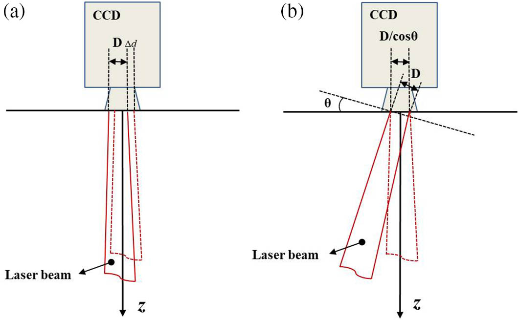
Figure 1.Top view along the $y$ axis of the simplified case, where the incident light beam carrying the OAM is in the $x - z$ plane. (a) Schematic illustration of the transversal displacement of a misaligned laser beam, where $D$ is the diameter of the laser beam spot, and $Δ d$ is the transversal displacement of a laser beam that has been shifted. (b) Schematic illustration of the tilt of a misaligned laser beam, where $θ$ is the tilt angle, and $D / \cos θ$ is the actual light spot diameter that is captured by the CCD when the tilt occurs.

For example, in free space optical communications, an acquisition, tracking, and pointing (ATP) system^[13] that reduces disturbances from atmospheric turbulence, platform shock, and alignment errors and improves communication efficiency has been introduced to handle these misalignments. The ATP system calculates the light spot coordinates in an image produced by a photodetector, such as a charge-coupled device (CCD) or a complementary metal–oxide–semiconductor (CMOS) detector, in real time. The most commonly used methods include the centroid algorithm^[14], the edge location algorithm^[15], the peak position algorithm, and the polynomial fitting algorithm. However, these algorithms were all proposed to handle Gaussian beams, and most of them lose both their accuracy and their stability in real scenarios. In addition, some work has been done in the field of misaligned OV beams. Lin et al.^[16] presented a theoretical proof and numerical simulations of a method to determine the misalignments of an OV beam, but without experimental verification. Huang et al.^[17] used the spiral phase structures of the OV measured using a Shack–Hartmann wavefront sensor to detect the phase center position of an OV beam; however, it was not the aim of their work to measure the misalignment of OV beams, and their optical system was too complex to handle some of the alignment issues.

An OV beam, unlike a Gaussian beam, consists of concentric rings with darkness at its center, and it suffers large-scale divergence during propagation, which causes a series of difficulties in the processes of positioning and tracking. In experimental situations in particular, an off-axis OV beam will occur in most cases, which will then lead to the asymmetry of the OV beam that reduces the accuracy of the other measurement algorithms^[18,19].

Sign up for Chinese Optics Letters TOC. Get the latest issue of Chinese Optics Letters delivered right to you！Sign up now

In this Letter, an experimental system and a related algorithm that we refer to as the cross-correlation method in the remainder of the paper are proposed to measure a misaligned OV beam, including its transversal displacement and tilt. Comparison of the results measured using our system with those from the numerical simulations shows the good performance of our method in determining the misalignments of the OV beam. In addition, our method can play a crucial role under different conditions and is suitable for use with both Gaussian beams and OV beams in both numerical simulation and experimental situations.

In cylindrical coordinates, the amplitude distribution of an LG beam is shown as follows^[20]: ${LG}_{pl} = \sqrt{\frac{2 p!}{π (p + | l |)!}} \frac{1}{w (z)} {[\frac{r \sqrt{2}}{w (z)}]}^{| l |} \exp [\frac{- r^{2}}{w^{2} (z)}] L_{p}^{| l |} [\frac{2 r^{2}}{w^{2} (z)}] \exp [\frac{i k_{0} r^{2} z}{2 (z^{2} + z_{R}^{2})}] \exp [- i (2 p + | l | + 1) \arctan (\frac{z}{z_{R}})] e^{i l θ},$ (1)where $r$ , $θ$ , and $z$ are the cylindrical coordinates, $k_{0}$ is the wavenumber, $l$ is the topological charge, $e^{i l θ}$ is the spiral wavefront phase factor, $p$ is the number of radial nodes in the intensity, and $λ$ is the wavelength of the beam. The radius of the Gaussian term is given by $w (z) = w (0) \times \sqrt{1 + {(\frac{z}{z_{R}})}^{2}}$ , where $z$ is the propagation distance, $z_{R}$ is the Rayleigh range, $w (0)$ is the beam waist, $(2 p + | l | + 1) \arctan (\frac{z}{z_{R}})$ is the Gouy phase, and $L_{p}^{| l |}$ is an associated Laguerre polynomial: $L_{p}^{| l |} (x) = \sum_{k = 0}^{p} {(- 1)}^{k} \frac{(p + l)!}{(p - k)! \times (k + l)!} \frac{x^{k}}{k!} .$ (2)

Using the mathematical equations given above, we simulate an LG beam with $p = 0$ , $l = 1$ , $λ = 633 nm$ , and $w (0) = 5 mm$ in a $1000 \times 1000$ pixel image. From Eq. (1), the spiral wavefront phase factor is the most prominent feature of the vortex beam. Because the OV beam propagates spirally, an uncertain phase singularity occurs at the center of the OV beam that forms a dark core with zero intensity at the center of the vortex.

In the numerical simulation of an OV beam, we can easily extract the required reference map from the image. However, in an experimental situation, the size of the light spot may differ from that in the simulated results. Therefore, using $w (0)$ and $λ$ , we first estimate the size of the OV beam that is imaged on a CCD or CMOS camera and then simulate an OV beam of the same size as that which was imaged by the camera. The size of the reference map is $401 \times 401$ under our experimental conditions, and a template with a center point is obtained.

An OV beam is generally produced by a Gaussian beam with a spiral wavefront phase. This beam inherits the properties of the laser beam. While there is some diffusion and deformation when an OV beam propagates in a medium, the intensity and shape of the beam remain almost entirely constant. Therefore, the results of cross-correlation operations between the template and the OV images with different misalignments can be determined stably and easily: $r = \frac{\sum_{m} \sum_{n} (A_{m n} - \bar{A}) (B_{m n} - \bar{B})}{\sqrt{[\sum_{m} \sum_{n} {(A_{m n} - \bar{A})}^{2}] [\sum_{m} \sum_{n} {(B_{m n} - \bar{B})}^{2}]}},$ (3)where A represents the matrix for the template, B is a matrix of the same size as A, and $\bar{A}$ and $\bar{B}$ are the average values of A and B, respectively. In addition, $m$ and $n$ are the dimensions of A. From Eq. (3), we can calculate the degree of correlation $r$ between A and B, i.e., the similarity of these two matrices. The $r$ value ranges from $- 1$ to 1, and a higher value of $r$ indicates greater similarity between the two matrices. We circulate the templates by performing the cross-correlation operation through an entire image that has a misalignment with respect to the original image; there will be a maximum value of $r$ because the shape and the intensity of the OV beam will not change too greatly during propagation. Finally, the distance between two images with the transversal displacement of the OV is calculated based on the location of the maximum value of $r$ .

The proposed algorithm to calculate the transversal displacement consists of three steps. In the first step, we simulate a reference map for an OV beam with a marked center, and a template, which shows great similarity to the reference map, is obtained by performing a cross-correlation using the appropriate algorithm between the reference map and the original OV image. In the second step, cross-correlation operations are performed through most of the pixels of the entire map that shows the transversal displacement using the previously prepared template. In the final step, the transversal displacement of the OV beam is the distance between the two points with the maximum values after the cross-correlation operation. When measuring the tilt of the OV beam, we use a series of templates with set angles to perform the cross-correlation operation with the OV maps that are to be tested. Using the LG beam as an example, we studied the LG beam intensity profile and then carried out an optical experiment to verify the proposed method. A specific illustration of the use of our algorithm is shown in Fig. 2.

Figure 2.Flowcharts for measurement of misalignments of the OV beam. (a) Transversal displacements of various OV maps as captured by our experimental setup and measured using the cross-correlation algorithm. A template of an OV beam is obtained by performing a cross-correlation between a reference OV map simulated according to the experimental conditions and an OV map with no transversal displacement. (b) The tilt of the OV map can be determined by simulating a set of OV templates with set tilt angles and then cycling them with OV maps that have a tilt obtained using our method.

An experimental setup was built to test our method, as illustrated schematically in Fig 3. A Gaussian beam emitted from a He–Ne laser (wavelength: 633 nm) was collimated after passing through a polarizer and a spatial filter (which consisted of an objective lens, a pinhole, and a collimating lens). The collimated beam was then incident on a prism that split the beam into two. One beam arrived at a reflective-type phase-only liquid crystal spatial light modulator (LCSLM), which transformed the incident light beam into an OV beam by displaying a spiral phase pattern on it; the beam then passed through the prism before finally arriving at a CCD camera that recorded the image of the OV beam, while the other beam was blocked by a blocker after it passed through the prism.

Figure 3.Schematic of the experimental setup. In our system, a collimated laser beam is reflected by the spatial light modulator (SLM) to form an OV beam, and its image is acquired by a CCD camera. Adjustment of the optical 3D translation platform or the rotating platform beneath the CCD is performed to generate transversal displacement or tilt, respectively. The polarizer and spatial filter are used to collimate the laser beam. The SLM is used to transform the laser beam into an OV beam. The prism is a beam splitter. The blocker is used to block the laser beam. The CCD is used to image the OV beams with the different misalignments.

An optical 3D translation platform or a rotation platform was placed beneath the CCD camera to obtain images of the different misalignments of the OV beam that were used to verify our algorithm. Here, we use the transversal displacement of the CCD camera rather than the translation of the entire light path because there is a relative motion between them. The minimum scale of the optical three-dimensional (3D) translation platform is $10 μ m$ . The LCSLM used in our experiments was a reflective-type phase-only modulation device, which had $512 \times 512$ pixels with pixel sizes of $16 μ m \times 16 μ m$ . The CCD camera had $1280 \times 1024$ pixels with pixel dimensions of $3.6 μ m \times 3.6 μ m$ .

To test the basic performance of the experimental system, we first observed images of the vortex beams generated by the LCSLM shown in Fig. 2. We used LG beams with $p = 0$ and $l = 1$ as examples. Typical donut-type intensity distributions with constant-intensity circular contours are clearly visible. We then cycled the reference map with a marked center, which contained extremely similar intensity distributions, as images captured using the CCD camera, through the entire image with the cross-correlation algorithm. Finally, by calculating the maximum value of the degree of correlation $r$ , we obtained the template for the OV beam with a known center under experimental conditions. The $r$ value of the numerical OV beam’s template and that of the experimental template are both approximately 0.9. These values are more or less identical, so we set the OV template’s center in the experimental scenarios using the same coordinate position as the numerical center.

Under ideal simulation conditions, we selected $1000 \times 1000$ pixels with OV beams ( $p = 0$ , $l = 1$ ) at the center of the image. We then used a series of OV beam images with known transversal displacements that were offset by 1, 2, 5, 10, 20, and 50 pixels.

In a similar manner, under the experimental conditions, a Gaussian beam emitted from a He–Ne laser passed through our experimental setup to form an OV beam. By translating the optical 3D translation platform with an $x$ orientation, we obtained a series of OV beam images with known transversal displacements, offset by minimum scales of 1, 2, 5, 10, 20, and 50.

Using the OV beam template that was obtained using the methods described above, we cycled our template through the series of OV images. We then compared the maximum values of $r$ to obtain the transversal displacement for each image. The results are extremely well matched with the preset offsets. We then elected some of the transversal displacement results shown in Fig. 4 to represent the experimental conditions, and the numerical curves of these results are shown to have great similarity.

Figure 4.Curves of cross-correlation of transversal displacements, where the red curve represents the original OV map with no transversal displacement, and the green curve is the OV map with the different transversal displacements. (a) Correlation coefficient curve for $10 μ m$ transversal displacement; (b) correlation coefficient curve for $20 μ m$ transversal displacement; (c) correlation coefficient curve for $50 μ m$ transversal displacement; and (d) correlation coefficient curve for $100 μ m$ transversal displacement.

By calculating the maxima of the red and green curves, we can obtain the transversal displacements of the OV beams. The results obtained under the numerical conditions are perfectly matched with the preset offsets. The offsets that were calculated under the experimental conditions are 3, 6, 14, 29, 58, and 140. By multiplying these results by the minimum size of one pixel of the CCD camera, which is 3.6 µm, we obtained corresponding final transversal displacements of 10.8, 21.6, 50.4, 104.4, 208.8, and 504 µm, respectively, which were well matched with the true values to a large extent.

Therefore, we obtained one pixel displacement resolution at the numerical simulation conditions and $10 μ m$ resolution according to the minimum scale of the optical translation platform under an experimental environment. Limited by an experimental equipment, we should have achieved higher resolution by using a smaller pixel size of the detector to achieve higher transversal displacement resolution.

Tilt determination is slightly different to transversal displacement detection, but we can also use our proposed algorithm to measure tilt. Figure 2(b) shows the different tilts of an OV beam. Under numerical conditions, we can simulate various tilt values of an OV beam. Reference [21] has previously clarified the mathematical derivation and presented a schematic diagram of a laser beam that happened to tilt. The interaction zone between the laser radiation and the accepting surface is formed elliptically because of the nonperpendicular angle of incidence. Here, we use an optical rotation platform to change the angle of the CCD camera surface. The absolute change in spot diameter $D^{*}$ is directly dependent on the inclination angle and the original spot diameter D. $D^{*}$ is calculated using $D^{*} = D \frac{1}{\cos θ} .$ (4)

Under numerical conditions, we can set a group of OV beams with different tilts so that we can detect various tilt angles by finding the maximum value of $r$ after using our method. However, under the experimental conditions, because of the limitations of the field of view of the CCD camera, we can hardly detect the complete OV beam beyond the angular range of $0 - π / 6$ . Additionally, we can even intuitively see that when the tilt is less than $π / 12$ , the deformation of the OV beam is difficult to determine, and our algorithm fails to detect these tilts. However, as the tilt angle increases, we can determine the tilts easily and reliably use our method. The brief operating steps are as follows: we use the optical rotation platform to rotate the CCD camera and then obtain the OV beam images at different tilt angles. We selected tilts of 15°, 20°, 25°, and 30° as examples to verify our method, as shown in Fig. 5.

Figure 5.Curves of the cross-correlation of tilt, where the green curve represents the OV map with specific angles produced by cycling our algorithm with the reference maps of different tilts ranging from 15° to 35°, and where the maximum of each curve is marked using a red square. (a) Correlation coefficient curve of 15° tilt; (b) correlation coefficient curve of 20° tilt; (c) correlation coefficient curve of 25° tilt; and (d) correlation coefficient curve of 30° tilt.

From Fig. 5, we see that our algorithm can determine the tilt by calculating the maximum value of $r$ , but there are also some errors that were mentioned above. When the tilt is small enough to cause our algorithm to lose its accuracy, as shown in Fig. 5(a), the maximum of $r$ does not occur when the tilt angle is 15°, while conversely, a smaller tilt angle leads to a larger value of $r$ . Additionally, Fig. 5(c) shows that when the tilt angle is 25°, the maximum of $r$ is 26°, with a 1° error that may be caused by the nonideal experimental OV map. Therefore, our algorithm still needs to be improved in terms of its stability and interference immunity for use in tilt determination. With the tilt angle around 20° or more, we can distinguish the tilt angle with resolution of about 1° ( $\sim 0.01 rad$ ).

While both transversal displacement and tilt would cause misalignment of the OV beam and introduce OAM spectrum dispersion, the latter is much more complex and critical.

The following part is focused on tilt determination. In fact, our method can handle different tilt situations. By simulating the OV reference maps for different types of tilt angle, we cycle the cross-correlation algorithm between these reference maps and the OV map captured using a CCD camera. After the maximal value of $r$ is calculated, the corresponding tilt angle can then be obtained. However, our method does not perform well in some cases. We therefore propose a solution to handle these issues. To simplify our process, we use the simplest case (tilt with $+ x$ orientation) as an example. It is well known that when the tilt angle of $θ$ occurs with $- x$ orientation, the OV image cannot be distinguished based on its intensity distribution, as detected using the CCD camera. Therefore, after the tilt angle is obtained by performing our method, we can rotate the optical rotation platform along the $x$ orientation. We can then observe the deflection of the OV beam, i.e., the ovality of the OV beam. Through judgment of the ovality of the OV map, we can easily determine the tilt angle with either $+ x$ or $- x$ orientation.

Another problem is that when the tilt angle is less than 20°, the method may lose its effectiveness. As shown in Fig. 5(a), the proposed algorithm demonstrated good performance in measuring the tilt angle over the range from 20° to 30°. Therefore, when a small tilt angle occurs, we can rotate the optical rotation platform at a fixed angle (which we set at 20°) so that the deflection of the OV map can obviously be detected using our algorithm. After following the same process used to determine the tilt angle that was described above, we obtain the final tilt by subtracting the fixed angle of 20°. Using the solutions presented above, our future work will aim to perfect our method, and we also intend to set up an OV reference map database so that we do not need to simulate the OV maps every time we use the method.

In summary, we have proposed a cross-correlation algorithm to determine the misalignment of an OV beam that includes transversal displacement and tilt under practical conditions when using some simple experimental equipment. The results showed high stability under various conditions and showed good agreement with the numerical simulation results; one pixel displacement of at least 0.01 mm was detected, and a tilt angle of approximately 0.01 rad was measured in our experiments. Because of the limitations of the experimental conditions, our method cannot measure all types of tilt. However, we have proposed some solutions to handle the shortcomings of our current algorithm. Additionally, our method shows good stability during the numerical simulations and is independent of the different misalignments of the OV beam (i.e., transversal displacement and tilt), which means that the proposed method can be used to determine these misalignments simultaneously.

References

[1] L. Allen, M. W. Beijersbergen, R. J. C. Spreeuw, J. P. Woerdman. Phys. Rev. A, 45, 8185(1992).

[2] L. Allen, M. J. Padgett, M. Babiker. Prog. Opt., 39, 291(1999).

[3] L. Allen, S. M. Barnett, M. J. Padgett. Optical Angular Momentum(2003).

[4] L. Tian, F. Ye, X. Chen. Opt. Express, 19, 11591(2011).

[5] M. Mirhosseini, M. Malik, Z. Shi, R. W. Boyd. Nat. Commun., 4, 2781(2013).

[6] W. Zhang, Q. Qi, J. Zhou, L. Chen. Phys. Rev. Lett., 112, 153601(2014).

[7] G. Gibson, J. Courtial, M. J. Padgett, M. Vasnetsov, V. Pas’ko, S. M. Barnett, S. Franke-Arnold. Opt. Express, 12, 5448(2004).

[8] Y. D. Liu, C. Gao, X. Qi, H. Weber. Opt. Express, 16, 7091(2008).

[9] M. Padgett, R. Bowman. Nat. Photon., 5, 343(2011).

[10] M. A. Lauterbach, M. Guillon, A. Soltani, V. Emiliani. Sci. Rep., 3, 2050(2013).

[11] G. Milione, T. Wang, J. Han, L. F. Bai. Chin. Opt. Lett., 15, 030012(2017).

[12] X. D. Chen, C. C. Chang, J. X. Pu. Chin. Opt. Lett., 15, 030006(2017).

[13] T. Jono, M. Toyoda, K. Nakagawa, A. Yamamoto, K. Shiratama, T. Kurii, Y. Koyama. Proc. SPIE, 3692, 41(1999).

[14] M. C. Amann, T. M. Bosch, M. Lescure, R. A. Myllylae, M. Rioux. Opt. Eng., 40, 10(2001).

[15] R. P. Mathur, C. I. Beard, D. J. Purll. Proc. SPIE, 1218, 129(1990).

[16] J. Lin, X. C. Yuan, M. Z. Chen, J. C. Dainty. J. Opt. Soc. Am. A, 27, 2337(2010).

[17] C. Huang, H. Huang, H. Toyoda, T. Inoue, H. Liu. Opt. Express, 20, 26099(2012).

[18] M. V. Vasnetsov, V. V. Slyusar, M. S. Soskin. Quantum Electron., 31, 464(2001).

[19] P. F. Ding, J. X. Pu. Acta Phys. Sin., 6, 031(2012).

[20] A. M. Yao, M. J. Padgett. Adv. Opt. Photon., 3, 161(2011).

[21] O. Pütsch, A. Temmler, J. Stollenwerk, E. Willenborg, P. Loosen. Proc. SPIE, 8843, 88430D(2013).