Temporal self-modifying characteristics of pulse propagation in multiphoton absorbers

Kun Cheng; Sujuan Zhang; Wei Li; Wanjun Dai; Dongxia Hu; Feng Jing

doi:10.3788/COL201513.070009

Abstract

In this Letter, temporal self-modifying behavior of amplitude modulation pulse propagation characteristics in multiphoton absorbers is presented by solving the underlying theoretical model coupling the propagation equation with the rate equations. The characteristics of the output temporal shapes are of primary concern and are discussed in detail. Amplitude modulation suppressing effects of multiphoton absorbers are numerically demonstrated; they have not been reported previously, to our knowledge. By taking a time resolved absorption coefficients, the corresponding physical mechanism is explicitly interpreted.

Multiphoton absorption (MPA) is a nonparametric process where an atom makes a transition from the ground state to a real state by simultaneously absorbing multiple laser photons. MPA materials and behaviors of organic materials induced by the MPA process have received increasing attention^[1–3]. Compared with other nonlinear absorption mechanisms, MPA has two distinct advantages. First, the transition probability for MPA depends on the laser intensity. Second, the temporal response of the nonlinear medium is fast because of the instantaneous nature of the MPA process. Such advantages enable the MPA materials to spatially control the excitation of a material in three dimensions and temporally modify the propagation characteristics of light in a medium with the light itself^[4]. The spatial controlling effect is demonstrated by applications such as 3D microfabrication^[5] and optical data storage^[6,7].

In the time domain, MPA materials have been used for pulse stabilization^[8] and pulse reshaping^[9]; Gao et al. have concerned the temporal pulse shape and verified the effects of excited state absorption on the pulse-shape distortion^[10]. However, the temporal modifying capability of MPA materials has not been explored. Coincidently, amplitude modulation is undesirable in both optical communication and laser fusion^[11] for adversely affecting the laser pulse performance. In this work, we investigated the dynamic process of an amplitude modulation pulse interacting with two-photon absorption (TPA) and three-photon absorption (3PA) in-depth by solving the basic theory model coupling the propagation equation with the rate equations. Great emphasis is placed on the evolution of the amplitude modulation, in which TPA and 3PA are compared with each other in detail.

The incident nonuniform beam is assumed with the following intensity profile $E (r, 0, t) = E_{0} \exp (\frac{- t^{8}}{2 T_{0}^{8}}) [1 + m \sin (2 π f_{m} t)] \exp (\frac{- r^{8}}{2 a_{0}^{8}}),$ (1)where t is time, r is radius, $E_{0}$ is the peak electric field, $a_{0}$ is the spatial beam waist, $T_{0}$ is the half-width of the 1/e temporal intensity, $m$ is the modulation depth, and $f_{m}$ is the modulation frequency. The modulation characteristics can be primarily determined by both $m$ and $f_{m}$ . In order to quantify the modulation degree, a conventional criterion by using the following is introduced^[12] $R = 2 \frac{I_{\max} - I_{\min}}{I_{\max} + I_{\min}} .$ (2)where $R$ is modulation degree and I is intensity.

Sign up for Chinese Optics Letters TOC. Get the latest issue of Chinese Optics Letters delivered right to you！Sign up now

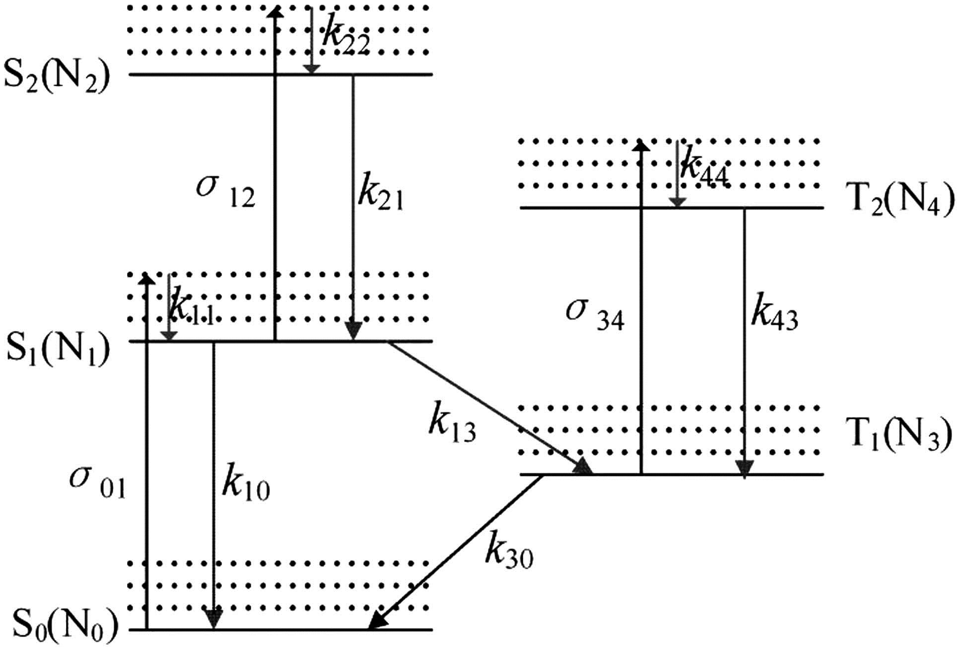
The molecular energy level structure of the selected TPA and 3PA materials is similar with a five-level model involving singlet and triplet states^[13], as shown in Fig. 1. Terms $S_{p}$ and $T_{p}$ represent a singlet state and a triple state, respectively. Term $σ_{p q}$ is the absorption cross section for electron transition from state $p$ to state $q$ , and $k_{p q}$ is the decay rate from state $p$ to state $q$ which are related to the decay time $τ_{p q}$ as $k_{p q} = τ_{p q}$ . Term $N_{p}$ is the electron number density of the state $p$ . The initial population density (i.e., chromophore concentration) $N_{T}$ is conserved such that $N_{0} + N_{1} + N_{2} + N_{3} + N_{4} = N_{T}$ .

Figure 1.Schematic diagram of a general five-level chromophore.

The propagation of the electric field along the $z$ -axis due to diffraction and various absorption processes from the participating levels is given by^[10,14–16] $(k_{1} \frac{\partial}{\partial t} + \frac{\partial}{\partial z}) E = - \frac{1}{2} (σ \cdot N) E .$ (3)The propagation distance is much shorter than the diffraction length. The diffraction is neglected in simulation. Additionally $σ \cdot N (r, z, t) = σ_{MPA} E^{2 (M - 1)} (r, z, t) N_{0} (r, z, t) + σ_{12} N_{1} (r, z, t) + σ_{34} N_{3} (r, z, t),$ (4)where $M$ denotes the number of photons absorbed by the ground state. Considering only absorption and relaxation processes, namely, ignoring coherent effects, the electronic state populations can be described by the rate equations^{[13,15,17,18]} $\frac{\partial N (r, z, t)}{\partial t} = [D_{0} + \sum_{M = 2,3} \frac{D_{M}}{M ℏ ω_{0}} E^{2 M} (r, z, t)] N (r, z, t),$ (5)where $N = [N_{0}, N_{2}, \dots, N_{4}]^{T}$ is a population density vector function $N (r, z, t)$ for a system with five electronic levels; $D_{0} \equiv D_{0} ([k_{p q}]), D_{1} \equiv D_{1} ([σ_{p q}]), D_{2} \equiv D_{2} ([σ_{TPA}])$ , $D_{3} \equiv D_{3} ([σ_{3 PA}])$ are constant $5 \times 5$ sparse matrices of decay rates $k_{p q}$ , single photon $σ_{p q}$ , two-photon $σ_{TPA}$ , and three-photon $σ_{3 PA}$ absorption cross sections, respectively. For simplicity, the transformations $A = \frac{E}{E_{0}} ρ = \frac{r}{a_{0}} ξ = \frac{z}{k_{0} a_{0}^{2} / 2} τ = \frac{t - k_{1} z}{T_{0}},$ (6)are used to obtain the nondimensional equations $\frac{\partial}{\partial ξ} A = - δ (σ \cdot N) A,$ (7) $\frac{\partial N (ρ, ξ, τ)}{\partial τ} = T_{0} [D_{0} + \sum_{M = 2,3} \frac{D_{M}}{α ℏ ω_{0}} A_{0}^{2 M} {| A |}^{2 M} (ρ, ξ, τ)] N (ρ, ξ, τ),$ (8)where $ℏ$ is Planck’s constant divided by 2π $a p = (n_{2} ω_{0} A_{0}^{2} / c) k_{0} a_{0}^{2} / 2$ . Equations (7) and (8) represent the set of coupled equations used to simulate the interaction progress.

In the numerical computations, unless noted otherwise, we used the following parameters for the laser: $λ = 1053 nm$ ; $a_{0}$ = 5 mm; pulse duration, $T_{0}$ = 1.5 ns; peak input energy, 2 J; modulation frequency, 2 GHz; modulation depth, $m$ = 0.025. For TPA^[19] and 3PA^[20], the relevant parameters are listed in Table 1.

Parameters	TPA	3PA
σ3PA (cm6/W2)		5.369×10−39
σTPA (cm4/W2)	2.5×10−29
σ12 (cm2)	1.68×10−20
σ34 (cm2)	3.0×10−17
k10 (ns−1)	3.68
k21 (ps−1)	0.602
k13 (μs−1)	22.08
k30 (ms−1)	2.717×103
k43 (ps−1)	1.0×10−4
L (mm)	10	10
NT (cm−3)	1.2×1020	5.96×1020

Table 1. Values of Parameters Used in Our Work

View all Tables

For a material, the transition probability depends on the square of the incident laser intensity, namely, $M = 2$ in the underlying equations. The temporal shape of the output pulse is governed largely by electron oscillation between the ground ( $S_{0}$ ) and first excited state ( $S_{1}$ ). Together with Eqs. (6) and (7), the computed population of the ground state at the entrance region is presented in Fig. 2 as a function of time. The curve in Fig. 2 implies the population in $S_{1}$ oscillates with the intensity and the depletion of the ground level is almost negligible, resulting from the fast temporal response of TPA. Nevertheless, the absorption in the TPA process is determined by not only the population depletion but also the laser intensity. For an intuitive analysis, a dynamic absorption coefficient with the following is proposed $α_{TPA} (t) = σ_{TPA} E^{2 (M - 1)} (r, z, t) N_{0} (t) = σ_{TPA} I (r, z, t) N_{0} (t) .$ (9)

Figure 2.(a) Normalized population density on $S_{0}$ versus time; (b) corresponding absorption coefficient at entrance region, $r = 0$ .

The absorption coefficient curve corresponding to Fig. 2(a) is plotted in Fig. 2(b). Clearly, the absorption coefficients for the peak intensity are always larger than that for the valley; in other words, a time-resolved intensity transmittance is produced.

According to the time-resolved intensity transmittance, a valuable result is obtained in Fig. 3, in which the modulation decreases from an initial value of 10%–2.37%. The relationship between amplitude modulation and propagation distance is simulated as well in Fig. 4 (black solid line), from which we can see that although the modulations decrease continually, the downward trend becomes slower as the pulse propagates. It is well-known that the suppression capability is limited to the difference between $α$ for the peak and the valley intensity is given by $Δ α_{TPA} = N_{0} σ_{TPA} [I (p) - I (v)] .$ (10)

Figure 3.Intensity profile versus time of input and output pulse at $r = 0$ .

Figure 4.Modulation as a function of propagation distance at $r = 0$ , for $I_{0}$ and $0.5 I_{0}$ .

Equation (10) implies that $∆ α$ depends on the value of [ $I (p) - I (v)$ ]; more surprisingly, the modulation suppressing capability can be actually self-modified. The deeper the modulation of the incident pulse, the more effectively the modulation is suppressed. As the pulse propagates, the modulation is reduced gradually, resulting in the slower decreasing trend. In order to demonstrate the influence of the laser intensity on the suppressing capability, the relationship between the amplitude modulation and the propagation distance of a lower-intensity pulse with peak input energy 1 J is also shown in Fig. 4 (red dashed line), from which we can see that modulations of a low-intensity pulse decrease more slowly than that of a high-intensity pulse.

As for 3PA materials, $M$ is 3, and Eq. (9) can be rewritten as $α_{3 PA} (t) = σ_{3 PA} E^{2 (M - 1)} (r, z, t) N_{0} (t) = σ_{TPA} I^{2} (r, z, t) N_{0} (t) .$ (11)Since $α_{3 PA}$ is the square of the intensity dependence, the modulation of $α_{3 PA}$ is larger than that of $α_{TPA}$ (cf. Fig. 5), giving rise to a larger $∆ α_{3 PA}$ than $∆ α_{TPA}$ ; therefore, we can expect that the modulation suppressing capability of 3PA is greater. Figure 6 gives the corresponding intensity profile of the output pulse with a modulation of 1.25%, which is smaller than that of TPA. Figure 6 also implies that 3PA transmits more energy relative to that of TPA. The energy transmittances of 3PA and TPA are shown in Fig. 7(a), from which we can see that the absorption of 3PA is always smaller than TPA, while the modulation diminishment is larger than TPA [cf. Fig. 7(b)].

Figure 5.Dynamic coefficients for 3PA and TPA as a function of time at entrance region, $r = 0$ .

Figure 6.Intensity profile versus time of output pulse for 3PA at $r = 0$ .

Figure 7.(a) Transmission versus distance for 3PA and TPA; (b) modulation versus distance for 3PA and TPA.

In practical applications, high-energy transmittance is also desirable. Thus, a synthetic evaluation parameter “performance price ratio (PPR)” is introduced, which is defined as the ratio of the modulation diminishment to the energy loss as depicted in Fig. 8. We can see that the PPR of 3PA along the propagation distance is steeper than that of TPA; the PPR of 3PA is higher initially, yet decreases below that of TPA as the pulse propagates. This is primarily because the modulation in 3PA is so small that $∆ α_{3 PA}$ is also less than $∆ α_{TPA}$ when the pulse propagates more than 0.5 cm.

Figure 8.Ratio of the modulation diminishment to the energy loss versus distance.

In conclusion, the temporal evolutions of an amplitude modulation pulse in TPA and 3PA materials are studied in detail. Based on a time-resolved intensity transmittance, the modulation diminishes gradually as the pulse propagates. Being the square of the intensity dependence, 3PA can alleviate the amplitude modulation more efficiently with less energy loss than TPA.

References

[1] Y. Fan, Z. Jiang, L. Yao. Chin. Opt. Lett., 10, 071901(2012).

[2] W. Cheng, S. Zhang, T. Jia, J. Ma, D. Feng, Z. Sun. Chin. Opt. Lett., 11, 041903(2013).

[3] Y. Chen, H. Guo, W. Gong, L. Qin, H. Aleyasin, R. R. Ratan, S. Cho, J. Chen, S. Xie. Chin. Opt. Lett., 11, 011703(2013).

[4] P. Zhao, Y. Zhang, W. Bao, Z. Zhang, D. Wang, M. Liu, Z. Zhang. Chin. Opt. Lett., 8, 93(2010).

[5] M. Rumi, J. W. Perry. Adv. Opt. Photon., 2, 451(2010).

[6] J. H. Strickler, W. W. Webb. Proc. SPIE, 1398, 107(1990).

[7] D. A. Parthenopoulos, P. M. Rentzepis. Science, 245, 843(1989).

[8] J. H. Strickler, W. W. Webb. Opt. Lett., 16, 1780(1991).

[9] G. S. He, R. Gvishi, P. N. Prasad, B. A. Reinhardt. Opt. Commun., 117, 133(1995).

[10] G. S. He, L. Yuan, J. D. Bhawalkar, P. N. Prasad. Appl. Opt., 36, 3387(1997).

[11] Y. W. Gao, M. J. Potasek. Appl. Opt., 45, 2521(2006).