
Chao-Ying Zhao, Wei-Han Tan. Analytical solution of three-dimensional Fourier transform frequency spectrum for three-level potassium atomic gas [J]. Acta Physica Sinica, 2020, 69(2): 020201-1
- Acta Physica Sinica
- Vol. 69, Issue 2, 020201-1 (2020)
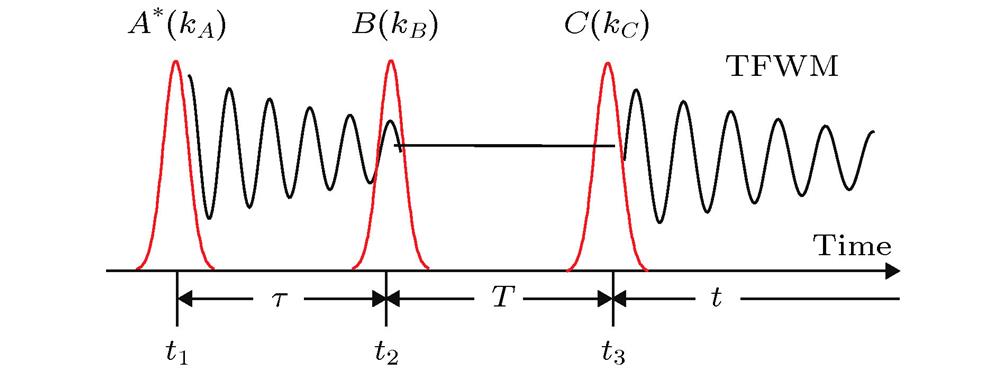
Fig. 1. Four wave mixing schematic.四波混频原理图
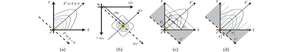
Fig. 2. (a) 2D time; (b) frequency coordinates for photon echo signals; (c) 2D time projection onto the diagonal corresponding to a slice along
; (d) 2D time projection onto the cross diagonal corresponding to a slice along
.
(a) 二维时域; (b) 光子回波信号的频率坐标; (c) 二维时域投影在对应于沿
的切片的对角线上; (d)沿
的切片对应的交叉对角线上的二维时域投影
Fig. 3. The three-dimensional Fourier transform spectrum
with
,
,
: (a) Real part; (b) imaginary part; (c) module.
当
,
,
时
频谱图 (a)实部; (b)虚部; (c)模
Fig. 4. The three-dimensional Fourier transform spectrum
with
,
,
: (a) Real part; (b) imaginary part; (c) module.
当
,
,
时
频谱图 (a)实部; (b)虚部; (c)模
Fig. 5. The three-dimensional Fourier transform spectrum
with
,
,
0.05 THz,
: (a) Real part; (b) imaginary part; (c) module.
当
,
,
,
时
频谱图 (a)实部; (b)虚部; (c)模
Fig. 6. The three-dimensional Fourier transform spectrum
with
,
,
0.05 THz,
(a) Real part; (b) imaginary part; (c) module.
当
,
,
,
时
频谱图 (a)实部; (b)虚部; (c)模
Fig. 7. Three-dimensional Fourier transform spectrum: (a) Fig. 5(a) in Ref. [11],
,
0.2 THz; (b)
; (c)
.
三维傅里叶转换频谱图 (a) 参考文献[11]中的图5(a) ,
,
, (b)
; (c)
Fig. 8. The three-dimensional Fourier transform spectrum with
,
,
for different R : (a)
; (b)
.
R 不同时, 三维傅里叶转换频谱,
,
,
(a)
; (b)
|
Table 1. The relation between in-homogeneous line-width and the diagonal correlation coefficient.

Set citation alerts for the article
Please enter your email address
© Copyright 2018-2021 | Chinese Laser Press. All Rights Reserved 沪ICP备15018463号-20