A convolution approach for the epilayer thickness in liquid phase epitaxial growth

Yan-Feng WEI; Quan-Zhi SUN

doi:10.11972/j.issn.1001-9014.2021.02.004

Abstract

The relation between the film thickness and the growth conditions in the liquid phase epitaxy (LPE) process is discussed. A convolution approach for the thickness is developed on the assumption that the growth rate is determined by the solute diffusion process. Using this convolution expression, the relations between thickness, growth time and cooling rate can be obtained for various LPE techniques. Moreover, the convolution algorithm can also be used to deal with some complex growth conditions, such as nonuniform cooling rate, nonlinearity of the liquidus curve and the finite growth solution.

Keywords

diffusion growth models liquid phase epitaxy

Introduction

As a mature technique for the growth of semiconductor films，Liquid Phase Epitaxy（LPE）has been widely used to grow III-V and II-VI semiconductor materials. In the LPE process，a substrate is inserted into the saturated solution and then the temperature of the system decreased while the solute crystallizes and deposits on the substrate to form a film. The thickness is the fundamental parameter of the film. Compared to Vapor epitaxy methods（MBE，MOCVD，etc.），it is usually difficult to monitor the thickness directly in the LPE process because the temperature of the growth solution is quite high and the growth crucible is opaque. So，it is essential to control the growth conditions carefully to obtain a designed film thickness.

Some factors that affect the epilayer thickness include the growth temperature，the growth time，the cooling rate，the Solid-Liquid phase diagrams，and so on. It is important to reveal the relation between the film properties and these factors. In the early study ^［1］，a diffusion equation was set up to describe the LPE process and it was demonstrated that the growth rate was mainly decided by the diffusion of the solute. An analytical solution was derived to describe the relation between the growth parameter and the growth rate in the semi-infinite boundary conditions. Henry T. Minden ^{investigated the details of the phase diagram and gave the solution of the diffusion equation in semi-infinite and bounded conditions^［2］. The question of constitutional supercooling was also presented in his study. R. L. Moon also studied the influence of thickness of growth solution on the LPE layer thickness and constitutional supercooling^［3］. Assuming the equilibrium concentration followed an Arrhenius law，Richard Ghez obtained an exact expression of the growth rate in unbounded condition^［4］. Muralidharan and S. C. Jain derived a more accurate solution of the diffusion equation in a solution with finite thickness and pointed out the discrepancy between the theory and the experiments was caused by the temperature variations of the diffusion coefficient of the solute^［5］. Crossley studied the LPE process using numerical method which was in principle adapted to various boundary conditions and cooling process^［6-8］. Besides these theoretical approaches，R. L. Moon，J. Kinoshita and J. J. Hsieh investigated the LPE of GaAs and compared the differences between the experiments and the theory^［9-10］. Their results demonstrated the epitaxial thickness calculated from the diffusion equation consisted with the experimental data. In the later studies^［11-15］，the numerical simulation methods were widely used due to the improvement of the computational ability. The contents investigated extended to 2-D，3-D and ternary alloy system. Meanwhile，the computational fluid method was adopted to study the influence of the melt convection on the epitaxial process.}

These studies were mostly based on the diffusion-limited model. The driving force of growth is the constitution gradient caused by the solute deposition in the cooling process. A constant cooling rate was mostly adopted in the theoretical models ^{［2-5，9-10］}. In their experiments，B. L. MOON and J. KINOSHITA ^［9］observed the discrepancy between the experimental data and the theoretical prediction. They ascribed these to the enhanced growth rate in the beginning of growth or thermal inertia of the growth furnace. In the LPE process，it is actually difficult to keep a constant cooling rate due to the ambient influence. The cooling rate will fluctuate around an average value，especially in a long-time growth process（one hour or more）. For this nonuniform cooling rate，the numerical method is preferred. However，an analytical model is more explicit and intuitive in the physical sense compared to the numerical method. In this paper，a convolution expression relating the film thickness to the growth time is derived based on the diffusion-limited model. The convolution algorithm could deal with bounded or unbound growth solution，nonuniform cooling rate，nonlinearity of the liquidus curve，and so on.

1 Theory

Assuming the thickness of the solution is $L$ ，the origin locates in the solid-liquid interface and the positive x direction points to the liquid，the LPE process could be described with the following diffusion equation，boundary，and initial conditions.^［1］

Diffusion equation：

\frac{\partial C (x, t)}{\partial t} = D \frac{\partial^{2} C (x, t)}{\partial x^{2}}

.（1）

Initial condition：

C (x, 0) = C_{0}

.（2）

Boundary condition：

\{\begin{matrix} C (0, t) = C_{l} (t) \\ \frac{\partial C (x, t)}{\partial x} |_{x = L} = 0 \end{matrix}

.（3）

With the semi-infinite growth solution， $L \to \infty$ ，the boundary condition Eq.3 changes to

Boundary condition：

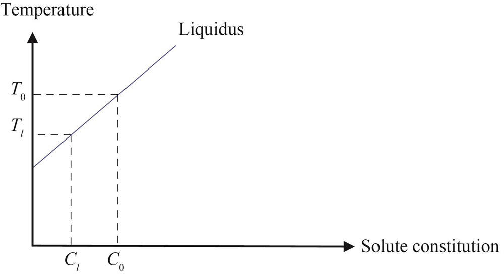
\{\begin{matrix} C (0, t) = C_{l} (t) \\ C (\infty, t) = C_{0} \end{matrix}

.（4）

Referring to Fig. 1， $C (x, t)$ is the concentration of the solution at the coordinates $x$ and the time $t$ ， $D$ is the diffusion coefficient of the solute， $C_{0}$ is the concentration of the initial solution， $T_{0}$ is the equilibrium temperature corresponding to $C_{0}$ ， $T_{l} (t)$ is the temperature on the solid-liquid interface at time $t$ . Assuming the solid-liquid two-phase keep equilibrium at the interface， $C_{l} (t)$ is then the solute concentration corresponding to $T_{l} (t)$ on the liquidus. In appendix A，a Laplace transform method is used to solve the Eqs.1-4 and the relation between the epilayer thickness and the growth time is obtained. Although the solving process is similar to that of in Refs.［2，9-10］except the developing of the convolution expression，a detailed derivation is given for the sake of clarity.

Figure 1.The schematic phase-diagram used in the LPE growth model

2 Discussion

In appendix A，the relation between the epilayer thickness and the growth time in the semi-infinite solution condition is given by

d (t) = \frac{1}{C_{s}} ∙ \sqrt[]{\frac{D}{π}} ∙ \frac{1}{\sqrt[]{t}} * [C_{0} - C_{l} (t)]

.（5）

The symbol * in Eq.5 is the convolution operator. So，the epilayer thickness is proportional to the convolution of the reciprocal of the square root of time and the “constitutional supercooling”. For different growth process，“constitutional supercooling” may have different form. J. J. Hsieh ^［10］classified the LPE process into four types which are Step-cooling，Equilibrium-cooling，Super-cooling and Two-phase solution technique. For the first three techniques，the relation between the epilayer thickness and the growth time can be described by the diffusion-limited model.

For the Equilibrium-cooling technique，the cooling rate $α$ is a constant. Assuming the slope of liquidus is also a constant $m$ ，it is obvious that $C_{0} - C_{l} (t) = \frac{T_{0} - T_{l} (t)}{m} = \frac{α t}{m}$ . So，

d (t) = \frac{1}{C_{s}} ∙ \sqrt[]{\frac{D}{π}} ∙ \frac{1}{\sqrt[]{t}} * (\frac{α t}{m}) = \frac{4}{3} ∙ \frac{1}{C_{s} m} ∙ \sqrt[]{\frac{D}{π}} ∙ α ∙ t^{\frac{3}{2}}

.（6）

For the Step-cooling technique，the degree of the supercooling $∆$ is a constant and $C_{0} - C_{l} (t) = \frac{∆}{m}$ . So，

d (t) = \frac{1}{C_{s}} ∙ \sqrt[]{\frac{D}{π}} ∙ \frac{1}{\sqrt[]{t}} * [C_{0} - C_{l} (t)] = \frac{1}{C_{s}} ∙ \sqrt[]{\frac{D}{π}} ∙ \frac{1}{\sqrt[]{t}} * (\frac{∆}{m}) = \frac{2}{C_{s} m} ∙ \sqrt[]{\frac{D}{π}} ∙ ∆ ∙ \sqrt[]{t}

.（7）

For the supercooling technique， $C_{0} - C_{l} (t) =$ $\frac{∆ + α t}{m}$ . So，

d (t) = \frac{2}{C_{s} m} ∙ \sqrt[]{\frac{D}{π}} ∙ (2 ∙ ∆ ∙ \sqrt[]{t} + \frac{4}{3} ∙ α ∙ t^{\frac{3}{2}})

.（8）

Equations 6-8 consist with those derived in Ref.［10］. For the widely used Equilibrium-cooling technique，the thickness is proportional to the time $t^{\frac{3}{2}}$ which means the growth rate of film increases gradually with time. It is possible to design a special cooling process in which the growth rate will be a constant. According to Eq.5，if the decrease of temperature is proportional to $t^{1 / 2}$ ，the film thickness will be proportional to time $t$ . In such cooling process，the growth rate is a constant which may benefit the uniformity of film and the simplicity of operation.

As for the two-phase-solution technique，the process deviates from equilibrium and the deposition will occur on both the substrate and the precipitates^［10］. The diffusion-limited model is not applicable for the two-phase-solution process.

Moreover，in appendix A，the epilayer thickness on the bounded solution condition is also obtained. On such conditions，the epilayer thickness is a sum of infinite series as described by Eq. A19. Supposing $C_{l} (t) = C_{0} - \frac{α t}{m}$ ，then the epilayer thickness can be calculated，

d (t) = \frac{α}{C_{s} m} ∙ [L t + \frac{2 L^{3}}{D} (\sum_{n = 0}^{\infty} \frac{e^{- \frac{D}{L^{2}} {(n + \frac{1}{2})}^{2} π^{2} t}}{{(n + \frac{1}{2})}^{4} π^{4}} - \frac{1}{6})]

.（9）

This result consists with that of obtained in Ref.［3］. So，Eq. 5 is a general one which can be simplified to various forms under different conditions.

As mentioned above，it is difficult to maintain a constant cooling-rate $α$ in a real growth process. The cooling-rate $α$ will change slightly during the cooling process. According to Eq. 6，we should get a straight line passing through the origin if we make a curve of $d (t)$ versus $t^{3 / 2}$ . However，the line did not always pass through the origin in the experiments. R. L. Moon etc. ^［9］ have observed this phenomenon. They thought the intercept would be positive if the growth rate was fast at the beginning of growth，while a negative intercept would occur if the cooling rate is small at the beginning due to the thermal inertia of the furnace. This non-uniform cooling process can be manipulated using Eq. 5. Assuming the slope of liquidus is a constant $m$ ，the degree of supercooling is $T_{s c} (t) = T_{0} - T_{l} (t) = [C_{0} - C_{l} (t)] ∙ m$ . Then，from Eq. 5，we can get：

d (t) = \frac{1}{C_{s} m} ∙ \sqrt[]{\frac{D}{π}} ∙ \frac{1}{\sqrt[]{t}} * T_{s c} (t)

.（10）

Numerically，the growth time $t$ is divided into N equal parts and the interval is $\frac{t}{N}$ for each part. The midpoint of each time interval is $t_{i} (i = 1,2 \dots N)$ . The degree of supercooling at moment $t_{i}$ is $T_{s c} (t_{i})$ . According to Eq. 10 and the definition of convolution，we get，

d (t) = \frac{1}{C_{s} m} ∙ \sqrt[]{\frac{D}{π}} ∙ \{\sum_{i = 1}^{N} \frac{T_{s c} (t_{i})}{\sqrt[]{t - t_{i}}}\} ∙ \frac{t}{N}

.（11）

In the above expression， $t_{i}$ and $T_{s c} (t_{i})$ are both measurable values. So，for this non-uniform cooling process，the numerical solution of the partial differential equation（PDE）is simplified to an algebraic sum.

As an example，the relationship between the temperature and the growth time in a HgCdTe LPE is shown in Fig. 2. The circle-solid line is the measured temperature. The decrease of the temperature is 6.5 $℃$ during the growth time of 63.5 minutes. The average cooling-rate is $α = 0.102 ℃ / m i n u t e$ . The dashed straight line is a supposed ideal cooling curve with a slope of 0.102 $℃ / m i n u t e$ . A deviation exists between these two curves which illustrates the cooling-rate is not a constant. The maximum deviation is about 0.5 $℃$ . The cooling-rate is small at the beginning，and it will change slightly during the whole growth process. If we suppose that the cooling-rate $α$ keeps constant as 0.102 $℃$ /minute in the growth process，we could get an epilayer thickness $d_{1}$ according Eq.6. Meanwhile，we can also calculate the thickness $d_{2}$ by adopting the real cooling curve in Fig. 2 and Eq.11. Finally，we get

\frac{d_{2}}{d_{1}} = \frac{\frac{1}{\sqrt[]{t}} * T_{s c} (t)}{\frac{4}{3} ∙ α ∙ t^{3 / 2}} = \frac{\{\sum_{i = 1}^{N} \frac{T_{s c} (t_{i})}{\sqrt[]{t - t_{i}}}\} ∙ \frac{t}{N}}{\frac{4}{3} ∙ α ∙ t^{3 / 2}} = 0.93

.（12）

Figure 2.The relation between temperature and the time in a LPE process

The above result means the real thickness will be smaller than the value calculated by Eq.6，the derivation of the thickness is about 7%. In Fig. 2，the real cooling curve is above the ideal cooling curve and takes a “convex” shape. This convex feature results in $d_{2} < d_{1}$ . If the real cooling curve is “concave”，the curve will be under the ideal cooling curve. Following the same calculation method，we will get $d_{2} > d_{1}$ .

In the LPE process illustrated in Fig. 2，we can also calculate the thickness variation with time according to Eq.11. The calculated results are shown in Fig. 3. In Fig. 3，the x-axis is the 3/2 power of time and the Y-axis is the nominal thickness in which assuming $\frac{1}{C_{s} m} ∙ \sqrt[]{\frac{D}{π}} = 1$ . The dashed-line is to guide the eyes. It can be seen the plot of the thickness versus $t^{3 / 2}$ is approximately a straight line except the first few data points. This straight line does not pass through the coordinate origin and gives a negative intercept. This result consists with that of obtained in Ref.［9］.

Figure 3.LPE layer thickness versus 3/2 power of growth time.

In the more general situation，the slope of the liquidus is not a constant. $C_{l}$ may be a function of temperature $T$ ， $C_{l} = C_{l} (T)$ . If the relation between temperature $T$ and time $t$ is $T = T (t)$ ， $C_{l}$ can be expressed as a function of time $t$ ， $C_{l} = C_{l} (T (t))$ . For instance，Henry T. Minden ^［2］ had supposed the relation between the solute concentration and the time near the solid-liquid interface is $C_{l} (t) = C_{0} e^{- \frac{t}{τ}}$ . Using Eq.5，we get

d (t) = \frac{1}{C_{s}} ∙ \sqrt[]{\frac{D}{π}} ∙ \frac{1}{\sqrt[]{t}} * [C_{0} - C_{l} (t)] = \frac{2 C_{0}}{C_{s}} ∙ \sqrt[]{\frac{D}{π}} ∙ [\sqrt[]{t} - \sqrt[]{τ} ∙ F (\sqrt[]{t / τ})]

,（13）

where $F (\sqrt[]{t / τ})$ is the Dawson function， $F (\sqrt[]{t / τ}) = e^{- t / τ} ∙ \int_{0}^{\sqrt[]{t / τ}} e^{y^{2}} d y$ .

3 Conclusions

The liquid phase epitaxy（LPE）process can be described by the diffusion-limited model. The convolution expression deduced in this study can deal with the three LPE techniques，namely step-cooling，equilibrium-cooling and supercooling. For the nonuniform cooling process，we compared the difference between the convolution calculation and the simply-model（uniform cooling-rate）calculation. The result shows there is a quite difference between these two methods which should be considered in the real LPE process. Moreover，by adopting the phase diagram data，the epilayer thickness could be predicted which is helpful to the control of LPE process.

References

[1] M B Small, J F Barnes. The distribution of solvent in an unstirred melt under the conditions of crystal growth by liquid epitaxy and its effect on the rate of growth. J. Crystal Growth, 5, 9-12(1969).

[2] H T Minden. Constitutional supercooling in GaAs liquid phase epitaxy. J. Crystal Growth, 6, 228-236(1970).

[3] R L Moon. The influence of growth solution thickness on the LPE layer thickness and constitutional supercooling requirement for diffusion-limited growth. J. Crystal Growth, 27, 62-69(1974).

[4] R Ghez. An exact calculation of crystal growth rates under conditions of constant cooling rate. J. Crystal Growth, 19, 153-159(1973).

[5] Muralidharan, S C Jain. Improvements in the theory of growth of LPE layers of GaAs and interpretation of recent experiments. J. Crystal Growth, 50, 707-719(1980).

[6] I Crossley, M B Small. Computer simulations of liquid phase epitaxy of GaAs in Ga solution. J. Crystal Growth, 11, 157-165(1971).

[7] I Crossley, M B Small. The application of numerical methods to simulate the liquid phase epitaxial growth of Ga1-xAlxAs from an unstirred solution. J. Crystal Growth, 15, 268-274(1972).

[8] M B Small, I Crossley. The physical processes occurring during liquid phase epitaxial growth. J. Crystal Growth, 27, 35-48(1974).

[9] R L Moon, J Kinoshita. Comparison of theory and experiment for LPE layer thickness of GaAs and GaAs Alloys. J. Crystal Growth, 21, 149-154(1974).

[10] J J Hsieh. Thickness and surface morphology of GaAs LPE layers grown by supercooling, step-cooling, equilibrium-cooling, and two-phase solution techniques. J. Crystal Growth, 27, 49-61(1974).

[11] S Y Leung, N E Schumaker. Layer thickness uniformity in liquid phase epitaxy: A two-dimensional diffusion analysis. J. Crystal Growth, 67, 458-466(1984).

[12] M Kimura, Z Qin, S Dost. A solid-liquid diffusion model for growth and dissolution of ternary alloys by liquid phase epitaxy. J. Crystal Growth, 158, 231-240(1996).

[13] I A Denisov, O S Mazhorova, Y P Popov et al. Numerical modelling for convection in growth/dissolution of solid solution CdXHg1-XTe by liquid-phase epitaxy. J. Crystal Growth, 269, 284-291(2004).

[14] Y C Liu, Z R Zytkiewicz, S Dost. A model for epitaxial lateral overgrowth of GaAs by liquid-phase electroepitaxy. J. Crystal Growth, 265, 341-350(2004).

[15] V V Kolmychkov, O S Mazhorova, Y P Popov. 3D computer simulation for convection in liquid phase epitaxy of ternary alloys. J. Crystal Growth, 303, 284-286(2007).