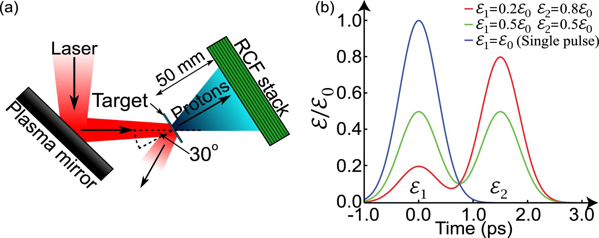
Fig. 1. (a) Schematic illustrating of the relevant aspects of the experimental setup. The incoming laser pulse is reflected from a plasma mirror before irradiating the target at $30^{\circ }$ incidence with respect to the target normal. The spatial profile and energy of the beam of accelerated protons are measured using a radiochromic film stack at the rear of the target. (b) Schematic of the idealized temporal profile of the incoming laser pulse for varying ${\mathcal{E}}_{1}$ and ${\mathcal{E}}_{2}$ energies.

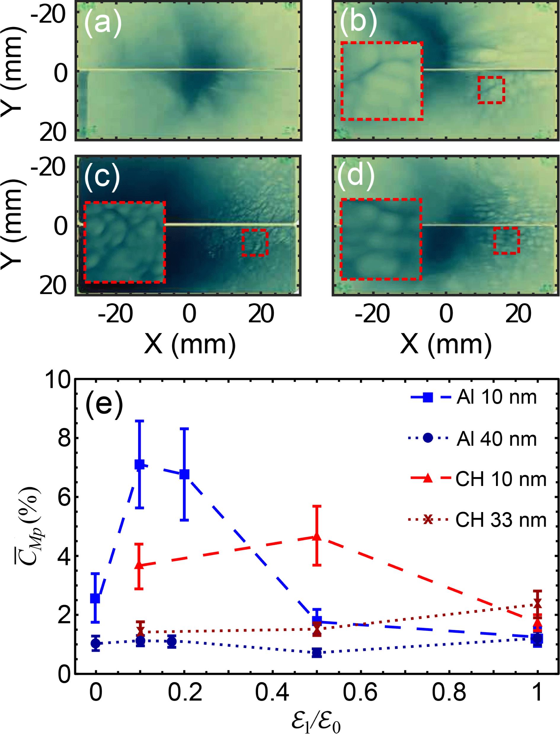
Fig. 2. Example proton spatial-intensity profile at 2.2 MeV for (a) ${\mathcal{E}}_{1}={\mathcal{E}}_{0}$, (b) ${\mathcal{E}}_{1}=0.01{\mathcal{E}}_{0}$, (c) ${\mathcal{E}}_{1}=0.1{\mathcal{E}}_{0}$ and (d) ${\mathcal{E}}_{1}=0.2{\mathcal{E}}_{0}$ for an $l=10~\text{nm}$ Al target. The dashed insets show a magnified region, highlighting the filamentary structures. (e) Degree of structure $\overline{C}_{Mp}$ present in the proton beam at 2.2 MeV as a function of ${\mathcal{E}}_{1}$ for stated foil thicknesses and materials.

Fig. 3. 2D simulation results at $t=-0.325~\text{ps}$ (where $t=0$ is the time when the peak of the first pulse reaches the target) for a laser pulse with ${\mathcal{E}}_{1}=0.1{\mathcal{E}}_{0}$ showing the spatial profile of (a) the transverse magnetic field, $B_{Y}$ and (b) the electron density, $n_{e}$. In all cases, the laser enters the simulation box from the left along the $x=0$ axis.

Fig. 4. 2D simulation proton density maps of the expanding rear proton layer for (a) ${\mathcal{E}}_{1}=0.01{\mathcal{E}}_{0}$ at $t=0~\text{ps}$ and (b) ${\mathcal{E}}_{1}=0.1{\mathcal{E}}_{0}$ at $t=-0.2~\text{ps}$. These example times are chosen such that there is a similar degree of proton layer expansion. (c) Time–space plot of proton density for ${\mathcal{E}}_{1}=0.1{\mathcal{E}}_{0}$ relative to the proton motion sampled along the transverse direction $0.25~\unicode[STIX]{x03BC}\text{m}$ from the rear edge of the proton layer. The white dashed line denotes the onset of RSIT. Note the density is normalized to the average proton density at each point in time to compensate for expansion.

Fig. 5. Time–space plot of the transverse magnetic field in the centre of the target ($Z=5~\text{nm}$) for a solid density, $l=10~\text{nm}$ Al target for (a) ${\mathcal{E}}_{1}=0.01{\mathcal{E}}_{0}$ and (b) ${\mathcal{E}}_{1}=0.1{\mathcal{E}}_{0}$. (c) and (d) Spatial Fourier transform of the magnetic field in (a) and (b), respectively.

Fig. 6. Plots of simulation results showing (a) formation time of the magnetic field structures as a function of ${\mathcal{E}}_{1}$, (b) longitudinal position, $Z$, of the back of the sheath-accelerated proton layer sampled at $X=0$ as a function of time, for each given ${\mathcal{E}}_{1}$, (c) longitudinal position, $Z$, of the rear of the expanding proton layer at $X=0$ (blue) and absolute azimuthal magnetic field strength (red) at the point in time at which the magnetic field structure formation begins as a function of ${\mathcal{E}}_{1}$, and (d) comparison of simulated and experimental proton $\overline{C}_{Mp}$ for an Al $l=10~\text{nm}$ target as a function of ${\mathcal{E}}_{1}$.