
Patrick Rambo, Jens Schwarz, Mark Kimmel, John L. Porter. Development of high damage threshold laser-machined apodizers and gain filters for laser applications[J]. High Power Laser Science and Engineering, 2016, 4(3): 03000e32
- High Power Laser Science and Engineering
- Vol. 4, Issue 3, 03000e32 (2016)
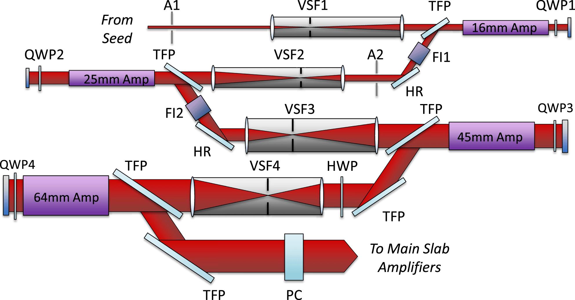
Fig. 1. Notional rod amplifier layout. A1 and A2 are apodizer and gain filter planes. VSF1, VSF2, VSF3 and VSF4 are vacuum spatial filters with 2.5x, 2x, 1.875x and 1.4x magnification respectively. TFPs are thin film polarizers. HRs are high reflector mirrors. QWP1, QWP2, QWP3 and QWP4 are zero-order quarter-wave plates while HWP is a zero-order half-wave plate. FI1 and FI2 are 12 mm and 25 mm Faraday isolators (which include a half-wave plate). PC is the final 75 mm clear aperture Pockels cell. Apodizer A2 defines an object plane for relay imaging, with image planes at the entrance to FI2 and the entrance to VSF4.
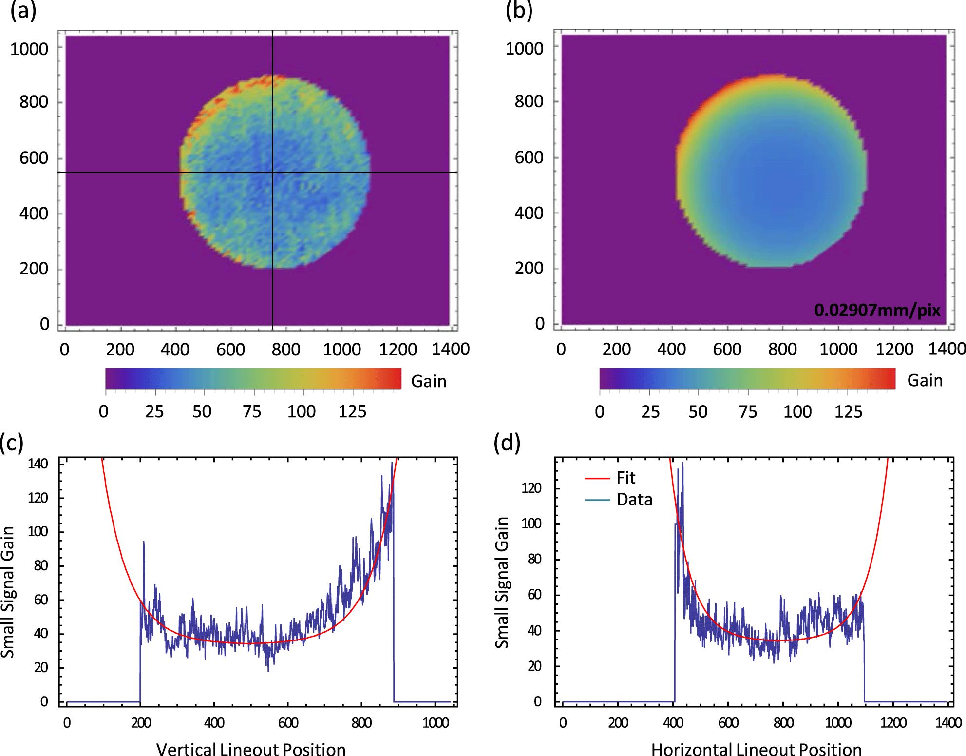
Fig. 2. Fits for double-pass small signal gain $G_{0}(r)$ for a 25 mm rod amplifier. (a) Measured 2D gain profile $G_{0}(r)$ at 64 mm near-field equivalent plane. (b) 2D fit to measured data using an asymmetrically placed exponentially decaying function. (c) Vertical lineout and fit. (d) Horizontal lineout and fit.
Fig. 3. Simulated spatial filtering of a dither pattern. (a) 2D continuous grayscale of ideal radial gain filter. (b) 2D error diffusion dither pattern (scale: $16~\text{mm}\times 16~\text{mm}$ ; pixel size: $40~\unicode[STIX]{x03BC}\text{m}\times 40~\unicode[STIX]{x03BC}\text{m}$ ). (c) Simulation of spatially filtered dither pattern. (d) False color view of the continuous filter image (a) subtracted from the dithered filtered image (c) with the scale shown relative to the peak of 1 in (a).
Fig. 4. Laser-machining setup. (a) Schematic. (b) Photograph.
Fig. 5. Sample laser-machined filters. (a) Sample Gain Filter (2 different sized samples on a 2 inch optic). (b) Sample Apodizer (5x microscope view).
Fig. 6. Sample performance of laser-machined gain filter. The false color image shows the spatially filtered near-field of a gain filter illuminated by a flat-top CW beam. Normalized horizontal and vertical lineouts (positioned on the respective centroids within the viewing aperture) are compared to the specified design (accounting for the area underfill issue mentioned in the text).
Fig. 7. Sample performance of laser-machined gain filter on amplified shot. The false color images are 12-bit near-field beam profile data taken after the 64 mm rod. The histograms show the counts at a given intensity value over the whole near-field image. (a) Left: Near-field to beam without soft-edged apodizer and gain filter; right: Histogram of unfiltered near-field data. (b) Left: Near-field to beam with soft-edged apodizer and gain filter; right: Histogram of filtered near-field data.

Set citation alerts for the article
Please enter your email address
© Copyright 2018-2021 | Chinese Laser Press. All Rights Reserved 沪ICP备15018463号-20