• High Power Laser Science and Engineering
  • Vol. 8, Issue 4, 04000e44 (2020)
I. Makos1、2, I. Orfanos1、2, E. Skantzakis1, I. Liontos1, P. Tzallas1、3, A. Forembski4, L. A. A. Nikolopoulos4, and D. Charalambidis1、3、*
Author Affiliations
  • 1Foundation for Research and Technology - Hellas, Institute of Electronic Structure & Laser, 70013Heraklion (Crete), Greece
  • 2Department of Physics, University of Crete, 70013Heraklion (Crete), Greece
  • 3ELI-ALPS, ELI-Hu Non-Profit Ltd., H-6720Szeged, Hungary
  • 4School of Physical Sciences, Dublin City University, Dublin 9, Ireland
  • show less
    DOI: 10.1017/hpl.2020.43 Cite this Article Set citation alerts
    I. Makos, I. Orfanos, E. Skantzakis, I. Liontos, P. Tzallas, A. Forembski, L. A. A. Nikolopoulos, D. Charalambidis. Strong-field effects induced in the extreme ultraviolet domain[J]. High Power Laser Science and Engineering, 2020, 8(4): 04000e44 Copy Citation Text show less

    Abstract

    Motivated by the achieved high intensities of novel extreme ultraviolet (XUV) radiation sources, such as free electron lasers and laser-driven high harmonic generation beamlines, we elaborate on their perspective in inducing observable strong field effects. The feasibility of extending such effects from the infrared and visible spectral regimes in the XUV domain is supported through numerically calculated models of near-future experiments. We highlight the advancement of performing studies in the time domain, using ultra-short XUV pulses, which allows for the temporal evolution of such effects to be followed. Experimental and theoretical obstacles and limitations are further discussed.

    1 Introduction

    The interaction of intense femtosecond (fs) laser radiation with atoms/molecules may lead to a substantial distortion of the atomic/molecular potentials and intrinsic dynamics. A well-known result of such a distortion is the so-called tunneling ionization that underlies processes such as high harmonic generation (HHG)[1] and above-threshold ionization (ATI)[2]. Tunneling ionization occurs when an infrared (IR) pulse is distorting the Coulomb potential of the system, forming potential barriers that oscillate with the laser period, through which an electron can tunnel out into the continuum. Whether tunneling or multiphoton is the main mechanism of photoionization depends on the interplay between the radiation’s field strength, frequency, pulse duration as well as the ionization energy of the atom/molecule. The key parameter that defines the mechanism underlying a photoionization process is the Keldysh or adiabatic parameter[3]

     (1)
    with ${E_{\rm ion}}$ being the ionization energy and ${U}_p$ the ponderomotive potential[4], i.e., the mean kinetic energy of the oscillation of a free electron interacting with the radiation field
     (2)
    where $m$ and $e$ are the mass and charge of the electron, respectively, $x$ is its position, and ${E}_0$ and $\omega$ are the electric field amplitude and the angular frequency of the radiation, respectively. A practical form of Equation (2) is
     (3)

    If $\gamma \ll 1$ , favored by long wavelengths, tunnel ionization prevails. When $\gamma \gg 1$ , favored by short wavelengths, ionization has a multiphoton character. It is well established that in the extreme ultraviolet (XUV) spectral range, owing to the short wavelength of the radiation, ionization is a multiphoton process, as tunneling would require intensities higher than the ionization saturation intensity of the system, i.e., intensities at which the atom no longer exists having been practically fully ionized during the rising of the laser pulse. While tunneling ionization is a process that by its nature is excluded in the XUV spectral region, other strong field effects, affecting the intrinsic system potentials, start becoming feasible at the high intensities that XUV and X-ray sources can reach today. Thus, in resonant coupling schemes with a free electron laser (FEL) source, strong-field dressing of an autoionizing state[5], as well as ac-Stark shifts of resonances[6] has been demonstrated recently. In the present work, we describe perspectives in observing and utilizing off-resonance strong field effects that can be induced by an attosecond pulse train (APT) generated in an intense laser-driven table-top XUV source. We further discuss other, potentially feasible, coherent resonant strong XUV field effects that have so far only been investigated in the visible spectral region.

    2 Nonresonant strong XUV field effects

    In order to induce nonlinear effects in the XUV region a powerful source is required[7]. Recently, a 20 GW XUV attosecond (as) beamline has been demonstrated at Foundation for Research and Technology - Hellas (FORTH), a detailed description of which can be found in the work of Nayak et al.[8] and Makos et al.[9]. In this beamline $\approx 200$ μJ of XUV radiation, in the spectral region of $15$ $35$ eV, is emitted per pulse at the source when two xenon jets are used for the harmonic generation[8] or APTs of $\approx 100$ μJ train energy, fs envelope duration and ${\tau}_{\rm xuv}=650\pm 80$ as pulse duration are emitted when one xenon jet is used[9]. In this source, after generation, the XUV radiation is separated from the driving IR field through reflection of the XUV radiation by a silicon plate placed at the Brewster angle ( $\sim\!7{5}^{\mathrm{o}}$ ) of the IR radiation. In addition, a Sn filter of $150$ μm thickness absorbs any residual IR radiation and transmits 11th–15th harmonics, i.e., XUV photon energies between 17 and 24 eV. The XUV beam is subsequently impinging at almost normal incidence to a gold coated spherical mirror of $5$ cm foal length focusing the beam in a $2$ μm spot measured by imaging the focal area using an ion microscope[8]. At such conditions, intensities of the order of $4\times {10}^{15}$ W/cm ${}^2$ can be achieved at the focus of the XUV radiation[8,9]. Such intensities, according to Equation (3), result in ponderomotive shifts larger than $1$ eV, for the previously mentioned photon energies. This is a rough estimation of the energy shifts that one would observe in the photoelectron spectrum of the multiphoton ionization of an atom due to the ponderomotive potential[10]. Given that the spectral bandwidth of the harmonics that synthesize the APT is less than $1$ eV and the resolution of detecting methods (e.g., common magnetic bottle time of flight electron energy analyzers) is of the order of $100$ meV, such shifts should in principle be observable.

    A more accurate evaluation of the shifts due to the XUV radiation field strength is obtained by solving the helium time-dependent Schrödinger equation (TDSE). The radiation field used in the calculation modeled the temporal profile of the electric field with a Gaussian envelope,

     (4)
    where $\tau$ is the envelope duration and ${c}_q, {\phi}_q$ parameters determine the chirp and the phase of each harmonic, respectively. In the present case only three harmonics were considered with amplitude ratio $|\,{E}_{11}|^2:|\,{E}_{13}|^2:|\,{E}_{15}|^2=0.19:0.4:0.41$ . These field characteristics simulate those of the harmonic spectra generated in the attosecond S&T Laboratory of FORTH[8,9]. The calculated photoelectron energy spectra (PES) of the two photon ionization of He by the comb of 11th–15th harmonics at different XUV intensities, ranging from $4\times {10}^{14}$ W/cm ${}^2$ to $3\times {10}^{15}$ W/cm ${}^2$ are shown in the top graph of Figure 1. The first two peaks are attributed to three-photon, Raman-type, processes. Note also the double peak structures showing up in the spectrum for the higher intensity.

    PES of the two-photon He ionization by a pulse train of an envelope fs, pulse duration as, synthesized by the 11th–15th harmonics with relative intensities 0.19:0.4:0.41, respectively, for different total XUV intensities ranging from W/cm to W/cm (top plot); PES peak shifts as a function of the total XUV intensity in the interval ranging from 0 to W/cm (bottom plot).

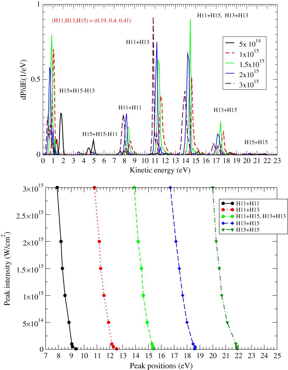
    Figure 1.PES of the two-photon He ionization by a pulse train of an envelope fs, pulse duration as, synthesized by the 11th–15th harmonics with relative intensities 0.19:0.4:0.41, respectively, for different total XUV intensities ranging from W/cm to W/cm (top plot); PES peak shifts as a function of the total XUV intensity in the interval ranging from 0 to W/cm (bottom plot).

    3 Resonant strong XUV field effects

    XUV EIT schemes in He through coupling of a bound with (a) an AIS or (b) two AISs.

    Figure 2.XUV EIT schemes in He through coupling of a bound with (a) an AIS or (b) two AISs.

    In an alternative ionization scheme, in order to better match the pulse duration with the width of the coupled states, the 5th harmonic of the SYLOS laser is resonantly coupling the 2s ${}^2$ $\;{}^1$ S AIS with the 25sp ${}^{+}$ $\;{}^1$ P AIS[27]. The 2s ${}^2$ $\;{}^1$ S AIS is near resonant with the 48th or even better harmonic in case surface plasma harmonics are used. The induced transparency can be investigated measuring either (a) the ion yield upon excitation of the 2s ${}^2$ $\;{}^1$ S and 25sp ${}^{+}$ $\;{}^1$ P AIS as a function of the 5th harmonic intensity or (b) the transmitted 48th harmonic as a function of the 5th harmonic intensity. A similar scheme has been investigated in Mg using visible laser radiation[28]. It should be noted that in this previous work it was shown that under appropriate conditions ionization can be diminished to a large percentage. This is an excellent perspective for the XUV spectral region where propagation in media is prohibited due to absorption that ionizes the medium. Switching off or, more realistically strongly suppressing ionization, opens up a possibility for the XUV radiation to propagate with strongly reduced intensity losses. Similar perspectives are opened up using all other coupling schemes discussed in this work. Similar EIT coupling schemes at lower photon energies can be implemented using other than He rare gases. To give an example, a scheme such as that shown in Figure 2(a) can be implemented in argon, where the 11th harmonic couples the 3s ${}^2$ 3p ${}^5$ ( ${}^2$ P ${}_{1/2}$ )4s state with the 3s ${}^3$ p ${}^6$ 4p ${}^1$ P ${}_1$ AIS.

    A VUV LICS scheme in He probed by an XUV field.

    Figure 3.A VUV LICS scheme in He probed by an XUV field.

    In all of the coupling schemes described previously, detuning is well within the bandwidth of the harmonics considered for the parameters of the ELI-ALPS SYLOS laser. The examples described previously can be implemented using variable delays between the two radiation fields, thus examining the dynamics of the effects and controlling the intensities used. From the technical point of view, the required two colors can be selected using either filters or multilayer mirrors. It is common practice in XUV delay lines that bisected reflecting optics are used. Different filtering coatings or different multilayer mirrors used in the two parts of the optics allow for selection of the required harmonics, while maintaining their pulse duration.

    Such types of experiments can of course be implemented in other laser laboratories as well, provided that the required XUV intensities and bandwidths are available and for certainty in FEL infrastructures. In fact, EIT-related experiments dealing with core resonant Auger decays have been modeled theoretically[29,30].

    4 Experimental considerations

    Successful implementation of the kind of experiments described in the previous sections is subject to bypassing a number of obstacles. Availability of high intensities is the first prerequisite. For FEL sources this is less of an issue. For laser-driven harmonic sources, high enough intensities are available in the low photon energy XUV spectral region, i.e., up to 25–30 eV. At higher photon energies there is a potential, but no experimental demonstrations exist at present.

    Photoelectron peak shifts observed with ionizing XUV intensity in single-photon ionization of Ar. Xe gas was utilized as the generating medium and a Sn filter was used for spectral selection. The spectra are obtained at two different XUV energies, measured by a calibrated XUV photodiode: 1.8 μJ/pulse (upper black line, shifted in y-axis for clarity), 0.5 μJ/pulse (lower blue line). The blueshifts are attributed to transient space charge induced on surfaces the direct or scattered XUV light is impinging.

    Figure 4.Photoelectron peak shifts observed with ionizing XUV intensity in single-photon ionization of Ar. Xe gas was utilized as the generating medium and a Sn filter was used for spectral selection. The spectra are obtained at two different XUV energies, measured by a calibrated XUV photodiode: 1.8 μJ/pulse (upper black line, shifted in y-axis for clarity), 0.5 μJ/pulse (lower blue line). The blueshifts are attributed to transient space charge induced on surfaces the direct or scattered XUV light is impinging.

    Harmonic spectra recorded by a flat-field XUV spectrometer (FFS) varying the peak gas density of Xe at the harmonic generation region: cm (upper black line, shifted in y-axis for clarity), cm (lower red line). The observed blueshift is of the order of eV.

    Figure 5.Harmonic spectra recorded by a flat-field XUV spectrometer (FFS) varying the peak gas density of Xe at the harmonic generation region: cm (upper black line, shifted in y-axis for clarity), cm (lower red line). The observed blueshift is of the order of eV.

    5 Theoretical challenges for ionization processes in XUV intense fields

    Following the introduction of the chirped-pulse amplification technique in the mid-1980s, the nonlinear interaction of atomic systems with visible laser fields has been studied extensively in great detail, both experimentally and theoretically. These studies resulted in the observation of a number of novel physical processes, such as ATI, HHG, and tunneling ionization. With the laser’s photon frequency relatively restricted to the long-wavelength scale (e.g., Ti:sapphire) the central factors allowing for these processes to show up experimentally are the strength and the ultrashort duration of the radiation field. In fact, ATI measurements require both intense ( $>{10}^{13}$ W/cm ${}^2$ ) and ultrashort pulses (femtosecond scale); fortunately, these characteristics go hand in hand. During the past two decades these studies have been extended to the UV/XUV regime in the wake of technological breakthroughs in producing intense, ultrashort and coherent radiation in this regime either using HHG or FEL generated radiation[37–39].

    Although the fundamental principles for the interaction of radiation and atomic/molecular systems remain the same as in the visible/IR regime, the relatively high-frequency (or shorter wavelength) of the XUV fields entails qualitatively and quantitatively distinct observations; some of them are so essential that they present certain experimental and theoretical challenges. An exclusive physical feature of the atomic interactions with fields of shorter wavelength is the possibility of excitation of inner-shell electrons (in the X-ray regime these are the prominent ionization channels); in contrast to the optical radiation where the excitation involves exclusively the valence electrons. In other words, the outer shell effectively constitutes an opaque shield for the inner-shell electrons against the visible/IR radiation. In contrast, the short-wavelength radiation at the higher-energy XUV regime, causes (with high probability) inner-shell or double-electron excitations to unstable continuum resonances, eventually leading to the system’s autoionization. Such a type of continuum excitation transitions can also be seen as ionization via an intermediate state (short-lived), which, depending on the atomic system and the radiation properties, perhaps competes with direct photoionization. It is also observed that for short-wavelength radiation, tunneling, ATI ionization and harmonic generation radiation are significantly suppressed.

    From a theoretical standpoint this wavelength regime necessitates a more detailed knowledge of the atomic structure, but on the other hand standard nonperturbative features of these interactions require very high intensities, not easily reached except in FEL facilities; for example, for the UV radiation ( $\omega >10$ eV) it appears that non-resonant processes can be rather adequately described by a time-dependent perturbation theory of the appropriate order for intensities lower than $5\times {10}^{14}$ W/cm ${}^2$ or, more generally, as long as the rate of ionization does not approach the field’s frequency. For higher intensities, ionization yield saturation, ac-Stark shifts, and the widths of the bound states start to play a noticeable role in the ionization process; such features may or may not be observable in the experimental data. Ultrashort pulses give a prominent role to the radiation’s detailed temporal profile owing to the extended power spectrum. The pulse may excite, resonantly and coherently, a number of bound or continuum atomic states that may cause the excitation dynamics to have a dominant role in the ionization process. The theoretical description of ionization dynamics with such ultrashort pulses requires a very cumbersome formulation when standard approximations are employed (i.e., time-independent/dependent perturbation theory, Floquet theory, etc.). Accordingly, relevant observations can be made for the radiation’s spatial distribution; for higher intensities, atoms in the laser focus experience ionization in shorter time scales than the atoms located in an extended region (where the intensity is lower). In addition, the experienced ac-Stark shifts can bring states on- and off-resonance in a highly complicated manner, resulting in analogously highly intricate ionization yields. In conclusion, one may argue that either due to the intensity or to the radiation’s temporal and spatial profile, observables of experimental interest are more reliably studied by direct employment of the TDSE. In the following we give an account of the TDSE description of atomic systems in XUV fields, followed by a brief adaptation of time-dependent perturbation equations of motion (EOMs) for potential XUV ionization schemes. For simplicity, for the presentation of the formulation we use the atomic system of units, where .

    5.1 TDSE

    In this context, the theoretical description (and the associated numerical algorithms and computational implementation) of nonlinear UV/XUV processes is a demanding problem. To date, such calculations using a broad range of radiation parameters, have been thoroughly performed only for hydrogen- and helium-like systems and with a lesser degree for the light noble gases, Ar and Ne.

    For the current purposes of UV/XUV fields, we briefly present the main expressions for the TDSE of an N-electron atomic system in a laser field, described by an electric field of a spatiotemporal profile, $\mathbf{E}\left(\mathbf{R},t\right)$ , in the Coulomb gauge ( $\mathbf{E}\left(\mathbf{R},t\right)=-{\partial}_tA\left(\mathbf{R},t\right),\kern0.5em {\nabla}_{\mathbf{R}}\mathbf{A}\left(\mathbf{R},t\right)=0$ ). Provided that a numerical representation of the atomic structure is available (in terms of the eigenenergies and the corresponding dipole matrix elements) and following a well-established calculation procedure[40–44] the TDSE is a partial differential equation that is second order in space and first order in time:

     (5)
    where ${H}_0$ is the field-free N-electron Hamiltonian, is the time-dependent wavefunction, and $\hat{V}\left(\mathbf{R},\mathbf{X};t\right)={\sum}_i\;\mathbf{A}\left(\mathbf{R},t\right)\cdot {p}_i$ describes the time-dependent potential experienced by the system at the position $\mathbf{R}$ . The electronic coordinates are defined relative to the system’s center-of-mass and denoted collectively by $\mathbf{X}=\left({\mathbf{r}}_1,{\mathbf{r}}_2,\cdots, {\mathbf{r}}_N\right)$ with the conjugate momenta defined by ${\mathbf{p}}_i=-\iota [{\hat{H}}_0,{\mathbf{r}}_i]$ . The separation of the atom/field Hamiltonian (right-hand-side of the TDSE) proves not only convenient for the numerical propagation of in time but also sets the prerequisites to developing a time-dependent perturbation theory; where the absolute value of the magnitude of the field-free part, ${H}_0=\,\mid {\hat{H}}_0\mid$ has to be larger than that of the time-dependent potential ${V}_0=\,\mid \hat{V}\mid \sim \mid \mathbf{A}\cdot \mathbf{p}\mid \sim {A}_0\mid [{\hat{H}}_0,r]\mid \sim {A}_0{H}_0{r}_0$ . To see this more clearly consider the expectation value of ${r}_0$ in the ground state of an atomic system, generally related to its energy by ${r}_0\sim 1/\sqrt{2 IP}$ . Then a perturbative method can be established as long as the following ratio is larger than unity:
     (6)
    Here ${E}_0={A}_0\omega$ is the maximum value of the electric field amplitude. Therefore, this ratio, is nothing else than the Keldysh parameter from Equation (1), which seen from an energy-domain aspect, serves as a parameter to establish the onset of a perturbative viewpoint.

    One method to calculate the solution of Equation (5) requires the expansion of the system’s time-dependent wavefunction on its eigenstates,

     (7)

    The eigenstates are characterized by the collective index, $K$ , to represent appropriate quantum numbers, i.e., the energy, angular, and spin quantum observables. The square amplitude of the time-dependent expansion coefficients, ${\left|{C}_K\left(\mathbf{R},t\right)\right|}^2$ , represents the probability of observing an atom (placed in an elementary volume at the tip of $\mathbf{R}$ ) in state at time $t$ (state populations). The differential equations for the coefficients are obtained by substituting Equation (7) into the TDSE (Equation (5)):

     (8)
    where ${V}_{K{K}^{\prime }}\left(\mathbf{R},t\right)$ are the dipole matrix elements between the states and . As can be seen, the TDSE depends on the system’s energies and the dipole matrix elements via its coefficients, with the former being constants and the latter being time-varying. Following this procedure, one is able to calculate experimental observables such as ionization yields, photoelectron kinetic and angular distributions, and harmonic yields. For example, the ionization yield at a given intensity, $I$ , is calculated at the end of the pulse by $Y(I)={\sum}_{E_K>0}{\left|{C}_K\right|}^2$ with ${E}_K>0$ used to select the system’s continuum states. The ionization yield originating from atoms inside the elementary volume ${V}_R$ is expressed as
     (9)
    where $\rho \left(\mathbf{R}\right)$ is the gas density and $Y[I(\mathbf{R})]$ is the yield from an atom placed at $\mathbf{R}$ , experiencing intensity $I\left(\mathbf{R}\right)$ . Obviously, a major part of solving the TDSE is in calculating the system’s electronic structure, a task which is not trivial going beyond the hydrogen, helium, and possibly lithium-like systems.

    A major simplification for the solution of Equation (8) is possible, because the wavelength of the UV/XUV pulse is much larger than the atomic scale. In this case one may solve the TDSE by dividing the interaction region into subregions of constant intensity, by setting fixed conditions on the $\mathbf{R}$ and then repeating the independent calculations for the individual volumes, ${{\rm d}V}_R$ . For example, for a Gaussian field in TEM ${}_{00}$ mode, ignoring the variation along the propagation axis, the intensity may be modeled by $I(r)={I}_0{e}^{-{r}^2/{w}_0^2}$ , where ${w}_0$ is the waist radius and $r$ the radial distance from the beam axis (z-axis). Then for ${\rm d}V\left(r,z=0\right)/ {\rm d}I=-{w}_0^2/I$ and constant gas density, ${\rho}_0$ , we obtain an expression for the yield:

     (10)

    Calculations that take into account the spatial distribution of the radiation beam are usually required when ionization saturation is starting to set in, as resonance conditions could be satisfied at various beam positions and time intervals. Accordingly, the time profile of the pulse (or, equivalently, the frequency spectrum) may cause time-dependent resonance conditions. The calculations shown in Figure 1 provide the photoelectron energy distributions for various intensities by solving the TDSE of helium in the pulse train discussed in Section 2. In these calculations no volume integration (in the sense of Equation (10)) has taken place. Thus, they represent the ionization yield produced at the pulse focus.

    5.2 Time-dependent perturbation theory

    Depending on the experimental conditions that include the setup, the radiation field, and the atomic system, simplifications of the TDSEs may be possible, namely by employing a perturbative formulation. Apart from the relative strength between the interaction potential and the atomic energies (see discussion around Equation (6)), another prerequisite for a time-dependent perturbative approach is a slow and fast time-varying factorized time profile for the field, the slow factor being the field’s envelope and the fast factor oscillating with the carrier-envelope frequency, $\omega$ :

     (11)

    The condition for slow and fast variation is mathematically expressed by ${\dot{\mathrm{\mathcal{E}}}}_0(t)\ll \omega {\mathrm{\mathcal{E}}}_0(t)$ . A linear combination of such pulses as the train forms in Equation (4) is less convenient to develop a perturbation theory as the number of terms increases.

    To demonstrate in what way the TDSEs are simplified we apply a perturbative treatment in the ionization scheme depicted in Figure 2(a). One can have as its starting point the EOMs of Equation (8) and develop a time-dependent perturbation resonant ionization theory by isolating the equations for the ground state $\mid\!g\rangle$ , the excited bound state, $\mid\!i\rangle$ , the AIS state, $\mid\!a\rangle$ , ${E}_g<{E}_i<0<{E}_a$ and the continuum states $\mid\!K\rangle, \,{E}_K>0$ . In this particular case of helium, $\mid\!g\left\rangle =\mid\!\!1{\rm s}^{2\;1}{\rm S}\right\rangle$ , $\mid\!i\left\rangle =\mid\!\!1{\rm s3{p}\ {}^1P}\right\rangle$ , $\mid\!a\left\rangle =\mid\!2{\rm p}^{2\;1}{\rm S}\right\rangle$ , and $\mid\!K\left\rangle =\mid\!\!1{\rm s}{\it E}_{\it K}{\rm p}\ {}^1{\rm P}\right\rangle$ . To exploit experimental data for AISs, one can develop the EOMs in a Fano-representation picture where the AIS parameters are compactly described by their ${q}_a$ -Fano parameter and autoionization decay width, (see Ref. [25]). One can also choose a formulation where a system of ordinary differential equations (ODEs) for the amplitudes is derived for the associated density matrix element of the system’s time-dependent state, defined by ${\sigma}_{K{K}^{\prime }}(t)={e}^{i\left({E}_K+\omega -{E}_{K^{\prime }}\right)}{C}_K(t){C}_{K^{\prime}}^{\ast }(t)$ . Although this is not the place to elaborate on the details of the derivation of the equations, it suffices to say that one arrives at a system of low number of ODEs for the states in question by effectively eliminating the time evolution of the continuum states; the interaction of the radiation with the continuum states is represented in the EOMs implicitly via the induced ionization widths and the ac-Stark shifts that are directly related to the field’s intensity[45,46]. It is worth noting here that the density-matrix formulation can be applied to a more diverse range of ionization schemes which include strongly fluctuating (i.e., FELs) and/or unpolarized radiation, florescence transitions, etc. In the case of ionization as described in Figure 2(a) we have

     (12a)
     (12b)
     (12c)
     (12d)
     (12e)

    In these equations, ${\gamma}_i(t)$ is the total ionization width of the state $\mid\!i\rangle$ due to both fields, is the time-dependent Rabi transition amplitude, and is the complex Rabi transition amplitude between the first excited state $\mid\!i\rangle$ and the AIS $\mid\!a\rangle$ . Here ${\mathrm{\mathcal{E}}}_1(t), \,{\mathrm{\mathcal{E}}}_2(t)$ are the field’s envelopes and ${\mu}_{gi}, \,{\mu}_{ia}$ represent the dipole matrix elements between the respective Fano states. In these equations, and are the detuning of the laser field where ${\overline{E}}_a={E}_a+{S}_a$ and ${\overline{E}}_i={E}_i+{S}_i$ are the effective energies which include the ac-Stark shifts ${S}_a$ and ${S}_i$ of the states. More generally, the induced ac-Stark shift for a bound state, $\mid\!i\rangle$ , in the presence of a radiation field of central frequency, $\omega$ , and envelope, $\mathrm{\mathcal{E}}(t)$ , coupled with the states $\mid\!f\rangle$ (bound or continuum), is given by

     (13)
    where ${\omega}_{if}={E}_i-{E}_f$ . The energy associated with a state inside the radiation field is proportional to the field’s intensity; with its actual value strongly dependent on the particular system and state via the ${\mu}_{if}\;\mathrm{and}\;{\omega}_{if}$ parameters. From the structure of this expression we see that, generally, for transitions leading deep into the continuum, the ac-Stark shift, compared with the ionization width (which is the other quantity and includes information about the ionization process), takes a relatively small value. This is not the case when the transitions lead close to resonant states (i.e., doubly excited, Auger states) or to the respective ionization threshold. Thus, we see that the ionization dynamics of the system are governed by these dynamical parameters, which need to be determined beforehand in order to solve the perturbative EOMs.

    Note that at this level of approximation, further transitions from the AIS to higher continuum states are not included because they are expected to only become significant at higher intensities. One therefore succeeds in reducing a highly demanding computational problem to a very manageable set of equations which, it is worth noting, is expressed through experimentally measured quantities (energies, shifts, q-parameters, widths). Following the solutions of the perturbative EOMs one may calculate the ionization yield as

     (14)

    Ionization of lithium with a radiation field around 73.1 eV (H47) couples two AIS states. The lower state decays to Li whereas the higher state decays to Li.

    Figure 6.Ionization of lithium with a radiation field around 73.1 eV (H47) couples two AIS states. The lower state decays to Li whereas the higher state decays to Li.

    The lithium in its ground state $\mid\!g\rangle =$ Li $\left(1{\rm s}^2,2{\rm s};{\kern0.1em }^2{\rm S}\right)$ is radiated by an XUV field. With an XUV photon energy and the highest peak intensity currently available, one can make the assumption that the two-photon ionization process has significantly less importance relative to single-photon ionization. The single-photon ionization will lead to the continuum state of Li ${}^{+}\left(1{\rm s}^2;{\kern0.1em }^1{\rm S}\right)$ and Li ${}^{+}\left(1{\rm s},2{\rm s};{\kern0.1em }^{1,3}{\rm S}\right)$ only, owing to restrictions imposed by the dipole selection rules. The ground state is also strongly coupled to the AIS $\mid\!i\rangle =$ Li $\left(\left\{1{\rm s};{\kern0.1em }^3{\rm P}(3)\right\}+\left\{1{\rm s},3{\rm s};{\kern0.1em }^1{\rm S},4{\rm p}\right\}\right)$ (see Refs. [47,48]). The latter AIS state $\mid\!i\rangle$ is also resonantly coupled to a higher AIS, $\mid\!a\rangle =$ Li $\left(2{\rm s},2{\rm p}^2;{\kern0.1em }^2{\rm S}\right)$ . A similar double resonance in resonantly enhanced multiphoton ionization (REMPI) scheme involving the ground, an excited bound and an autoionizing state of Xe has been investigated previously using optical frequencies[49].

    This is a particularly interesting scheme because the resonant coupling between the ground state, $\mid\!g\rangle$ and the first AIS, $\mid\!i\rangle$ , and also with the second AIS, $\mid\!a\rangle$ (double resonance), is possible with the same photon frequency, as ${E}_f-{E}_i\simeq {E}_i-{E}_g$ . Two-photon sequential ionization from the Li ground state to the Li ${}^{2+}$ is not considered as the step from Li ${}^{+}$ to Li ${}^{2+}$ proceeds only via two-photon absorption, E(Li ${}^{2+}$ )–E(Li ${}^{+}$ ) $\sim$ 75.1 eV $<\omega$ .

    It is also worth exploring the effects of Rabi coupling between the AIS on the ionization yield. As autoionization via the AISs competes with direct photoionization it is expected that the pulse duration relative to the half-life of the AISs plays a role here. These lifetimes are approximately fs and fs for the first and the second AIS, respectively. Recalling that the resonances are $\sim 73.129$ eV for $\mid\!g\left\rangle \leftrightarrow \mid\!i\right\rangle$ and $\sim\!73.351$ eV for $\mid\!i\left\rangle \leftrightarrow \mid f\right\rangle$ (note that the two-photon ionization resonance occurs for $\sim$ 73.24 eV photon energy, $\mid\!g\left\rangle \to \to \mid\!b\right\rangle$ ).

    Ionization of lithium with a radiation field around 73.1 eV (H47) coupling two AIS states. We plot the population ratios of Li/Li for various coupling strengths of and for peak intensity W/cm. The multiplication factor for the coupling is shown in the inset. Values for and can be found in Ref. [48].

    Figure 7.Ionization of lithium with a radiation field around 73.1 eV (H47) coupling two AIS states. We plot the population ratios of Li/Li for various coupling strengths of and for peak intensity W/cm. The multiplication factor for the coupling is shown in the inset. Values for and can be found in Ref. [48].

    6 Conclusions

    The high intensities, achieved recently, in both FEL and laser-driven attosecond facilities, in the XUV spectral region opened up the era of strong field effects in this short-wavelength part of the electromagnetic radiation spectrum. In this work, we addressed near-future perspectives of investigations in this area. Several effects, well found in the visible spectral regime, are extendable to the XUV range under the experimental conditions that exist today. Examples of such experiments, enabling control of processes and dynamics during the interaction of the radiation with matter as well as modifying the propagation properties of the XUV radiation in matter have been presented. Ab initio numerical modeling of some of these effects has demonstrated the observability of the effects at hand. At the same time, experimental obstacles and potential artifacts along with mitigation strategies have been elaborated. It is expected that the presented perspectives will motivate numerous near-future experimental campaigns in FEL and attosecond infrastructures.

    References

    [1] M. Ferray, A. L’huillier, X. F. Li, L. A. Lompre, G. Mainfray, C. Manus. J. Phys. B At. Mol. Opt. Phys., 21(1988).

    [2] P. Agostini, F. Fabre, G. Mainfray, G. Petite, N. K. Rahman. Phys. Rev. Lett., 42, 1127(1979).

    [3] L. V. Keldysh. Soviet Phys. JETP, 20, 1307(1965).

    [4] L. V. Keldysh. Phys. Rev. Lett., 16, 1054(1966).

    [5] C. Ott, L. Aufleger, T. Ding, M. Rebholz, A. Magunia, M. Hartmann, V. Stooß, D. Wachs, P. Birk, G. D. Borisova, K. Meyer, P. Rupprecht, C. D. C. Castanheira, R. Moshammer, A. R. Attar, T. Gaumnitz, Z.-H. Loh, S. Düsterer, R. Treusch, J. Ullrich, Y. Jiang, M. Meyer, P. Lambropoulos, T. Pfeifer. Phys. Rev. Lett., 123(2019).

    [6] T. Ding, M. Rebholz, L. Aufleger, M. Hartmann, K. Meyer, V. Stooß, A. Magunia, D. Wachs, P. Birk, Y. Mi, G. D. Borisova, C. d. C. Castanheira, P. Rupprecht, Z.-H. Loh, A. R. Attar, T. Gaumnitz, S. Roling, M. Butz, H. Zacharias, S. Düsterer, R. Treusch, S. M. Cavaletto, C. Ott, T. Pfeifer. Phys. Rev. Lett., 123(2019).

    [7] I. Orfanos, I. Makos, I. Liontos, E. Skantzakis, B. Major, A. Nayak, M. Dumergue, S. Kuehn, S. Kahaly, K. Varjú, G. Sansone, B. Witzel, C. Kalpouzos, L. A. A. Nikolopoulos, P. Tzallas, D. Charalambidis. J. Phys. Photon, 2(2020).

    [8] A. Nayak, I. Orfanos, I. Makos, M. Dumergue, S. Kühn, E. Skantzakis, B. Bodi, K. Varjú, C. Kalpouzos, H. I. B. Banks, A. Emmanouilidou, D. Charalambidis, P. Tzallas. Phys. Rev. A, 98, 66(2018).

    [9] I. Makos, I. Orfanos, A. Nayak, J. Peschel, B. Major, I. Liontos, E. Skantzakis, N. Papadakis, C. Kalpouzos, M. Dumergue, S. Kühn, K. Varju, P. Johnsson, A. L’huillier, P. Tzallas, D. Charalambidis. Sci. Rep., 10, 3759(2020).

    [10] L. Jönsson. J. Opt. Soc. Am. B, 4, 1422(1987).

    [11] C. J. G. J. Uiterwaal, D. Xenakis, D. Charalambidis, P. Maragakis, H. Schröder, P. Lambropoulos. Phys. Rev. A, 57, 392(1998).

    [12] K.-J. Boller, A. Imamoğlu, S. E. Harris. Phys. Rev. Lett., 66, 2593(1991).

    [13] O. A. Kocharovskaya, Y. I. Khani. Sov. Phys. JETP, 63, 945(1986).

    [14] B. Dai, P. Lambropoulos. Phys. Rev. A, 39, 3704(1989).

    [15] P. E. Coleman, P. L. Knight, K. Burnett. Opt. Commun., 42, 171(1982).

    [16] Y. I. Geller, A. K. Popov. Sov. J. Quantum Electron., 6, 883(1976).

    [17] Y. I. Geller, A. K. Popov. Sov. J. Quantum Electron., 6, 606(1976).

    [18] S. Cavalieri, R. Eramo, L. Fini, M. Materazzi, O. Faucher, D. Charalambidis. Phys. Rev. A, 57, 2915(1998).

    [19] S. Cavalieri, F. S. Pavone, M. Matera. Phys. Rev. Lett, 67, 3673(1991).

    [20] Y. L. Shao, D. Charalambidis, C. Fotakis, J. Zhang, P. Lambropoulos. Phys. Rev. Lett, 67, 3669(1991).

    [21] S. S. Dimov, L. I. Pavlov, K. V. Stamenov, Y. I. Heller, A. K. Popov. Appl. Phys. B, 30, 35(1983).

    [22] Y. I. Heller, V. F. Lukinykh, A. K. Popov, V. V. Slabko. Phys. Lett. A, 82, 4(1981).

    [23] O. Faucher, E. Hertz, B. Lavorel, R. Chaux, T. Dreier, H. Berger, D. Charalambidis. J. Phys. B, 32, 4485(1999).

    [24] B. W. Shore, D. Charalambidis, M. Shapiro, P. L. Knight, T. Halfmann, K. Bergmann, L. P. Yatsenko, O. Faucher, S. Cavalieri, P. Lambropoulos. Phys. Rev. Lett., 93(2004).

    [25] U. Fano. Phys. Rev., 124, 1866(1961).

    [26] O. Faucher, D. Charalambidis, C. Fotakis, J. Zhang, P. Lambropoulos. Phys. Rev. Lett., 70, 3004(1993).

    [27] L. Lipsky, A. Russek. Phys. Rev., 142, 59(1966).

    [28] N. E. Karapanagioti, O. Faucher, Y. L. Shao, D. Charalambidis, H. Bachau, E. Cormier. Phys. Rev. Lett., 74, 2431(1995).

    [29] L. A. A. Nikolopoulos, T. J. Kelly, J. T. Costello. Phys. Rev. A, 84(2011).

    [30] N. Rohringer, R. Santra. Phys. Rev. A, 77(2008).

    [31] M. Di Fraia, O. Plekan, C. Callegari, K. C. Prince, L. Giannessi, E. Allaria, L. Badano, G. de Ninno, M. Trovò, B. Diviacco, D. Gauthier, N. Mirian, G. Penco, P. R. Ribivc, S. Spampinati, C. Spezzani, G. Gaio, Y. Orimo, O. Tugs, T. Sato, K. L. Ishikawa, P.A. Carpeggiani, T. Csizmadia, M. Füle, G. Sansone, P. Kumar Maroju, A. D’Elia, T. Mazza, M. Meyer, E. V. Gryzlova, A. N. Grum-Grzhimailo, D. You, K. Ueda. Phys. Rev. Lett., 123(2019).

    [32] K. C. Prince, E. Allaria, C. Callegari, R. Cucini, G. de Ninno, S. Di Mitri, B. Diviacco, E. Ferrari, P. Finetti, D. Gauthier, L. Giannessi, N. Mahne, G. Penco, O. Plekan, L. Raimondi, P. Rebernik, E. Roussel, C. Svetina, M. Trovò, M. Zangrando, M. Negro, P. Carpeggiani, M. Reduzzi, G. Sansone, A.N. Grum-Grzhimailo, E. V. Gryzlova, S. I. Strakhova, K. Bartschat, N. Douguet, J. Venzke, D. Iablonskyi, Y. Kumagai, T. Takanashi, K. Ueda, A. Fischer, M. Coreno, F. Stienkemeier, Y. Ovcharenko, T. Mazza, M. Meyer. Nat. Photon., 10, 176(2016).

    [33] H. J. Shin, D. G. Lee, Y. H. Cha, J.-H. Kim, K. H. Hong, C. H. Nam. Phys. Rev. A, 63(2001).

    [34] H. J. Shin, D. G. Lee, Y. H. Cha, K. H. Hong, C. H. Nam. Phys. Rev. Lett., 83, 2544(1999).

    [35] C. Altucci, T. Starczewski, E. Mevel, C.-G. Wahlström, B. Carré, A. L’Huillier. J. Opt. Soc. Am. B, 13, 148(1996).

    [36] E. Constant, D. Garzella, P. Breger, E. Mével, C. Dorrer, C. Le Blanc, F. Salin, P. Agostini. Phys. Rev. Lett., 82, 1668(1999).

    [37] P. Tzallas, E. Skantzakis, L. A. A. Nikolopoulos, G. D. Tsakiris, D. Charalambidis. Nature Phys., 7, 781(2011).

    [38] P. K. Maroju, C. Grazioli, M. Di Fraia, M. Moioli, D. Ertel, H. Ahmadi, O. Plekan, P. Finetti, E. Allaria, L. Giannessi, G. de Ninno, C. Spezzani, G. Penco, S. Spampinati, A. Demidovich, M. B. Danailov, R. Borghes, G. Kourousias, Dos Reis C. E. Sanches, F. Billé, A. A. Lutman, R. J. Squibb, R. Feifel, P. Carpeggiani, M. Reduzzi, T. Mazza, M Meyer, S. Bengtsson, N. Ibrakovic, E. R. Simpson, J. Mauritsson, T. Csizmadia, M. Dumergue, S. Kühn, H. Nandiga Gopalakrishna, D. You, K. Ueda, M. Labeye, J. E. Bækhoj, K. J. Schafer, E. V. Gryzlova, A. N. Grum-Grzhimailo, K. C. Prince, C. Callegari, G. Sansone. Nature, 578, 386(2020).

    [39] N. A. Papadogiannis, L. A. A. Nikolopoulos, D. Charalambidis, G. D. Tsakiris, P. Tzallas, K. Witte. Appl. Phys. B, 76, 721(2003).

    [40] H. Bachau, E. Cormier, P. Decleva, J. E. Hansen, F. Martín, Rep. Prog. Phys., 64, 1815(2001).

    [41] E. Foumouo, A. Hamido, P. H. Antoine, B. Piraux, H. Bachau, R. Shakeshaft. J. Phys. B, 43(2010).

    [42] P. Lambropoulos, L. A. A. Nikolopoulos. New J. Phys., 10(2008).

    [43] L. A. A. Nikolopoulos, T. Nakajima, P. Lambropoulos. Phys. Rev. Lett., 90(2003).

    [44] L. A. A. Nikolopoulos, T. K. Kjeldsen, L. B. Madsen. Phys. Rev. A, 75(2007).

    [45] B. W. Shore. The Theory of Coherent Atomic Excitation(1990).

    [46] P. Lambropoulos, P. Zoller. Phys. Rev. A, 24, 379(1981).

    [47] K. T. Chung, B.-C. Gou. Phys. Rev. A, 52, 3669(1995).

    [48] D. Middleton. The development of a theoretical and computational framework of ultrafast processes of complex atomic systems in a strong radiation field,(2014).

    [49] D. Charalambidis, J. A. D. Stockdale, C. Fotakis. Z. Phys. D, 32, 191(1994).

    I. Makos, I. Orfanos, E. Skantzakis, I. Liontos, P. Tzallas, A. Forembski, L. A. A. Nikolopoulos, D. Charalambidis. Strong-field effects induced in the extreme ultraviolet domain[J]. High Power Laser Science and Engineering, 2020, 8(4): 04000e44
    Download Citation