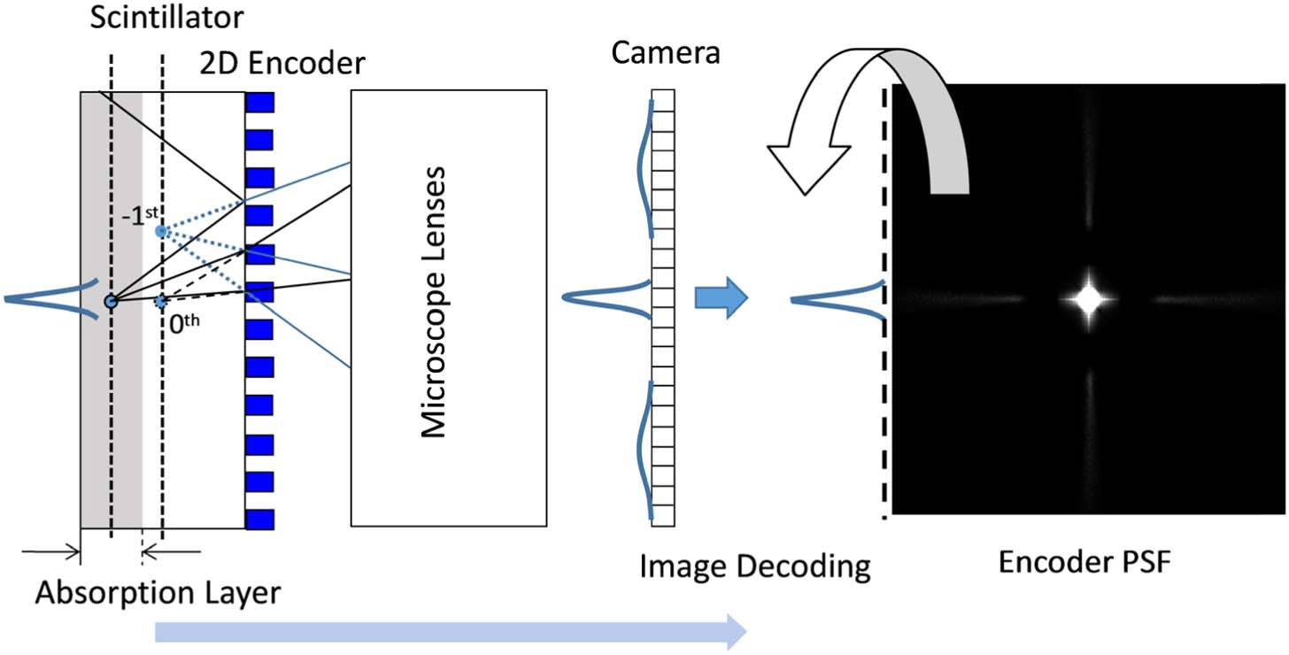
Fig. 1. Schematic of an X-ray scintillator imager based on the use of the proposed high-spatial-frequency spectrum enhanced reconstruction (HSFER) method. A two-dimensional (2D) encoder is used to extract the middle-high-frequency and high-frequency components of the image generated in the scintillator. The image is decoded by a PSF/OTF of the encoder.

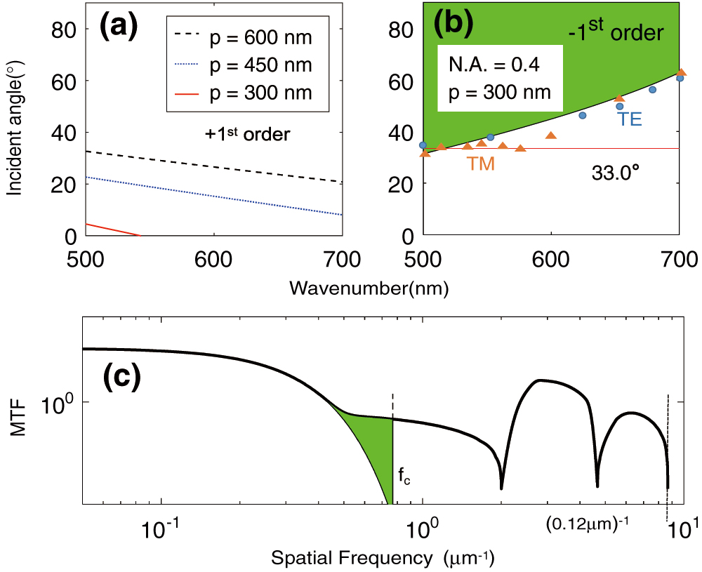
Fig. 2. (a) Areas below the dashed, dotted, and solid curves represent the parameter zones that allow the +1st-order diffraction to occur for the two-dimensional (2D) encoder periods of 600, 450, and 300 nm, respectively. This shows that the encoder with a 300 nm period can yield a maximum suppression of the +1-order diffraction compared with the other two encoders. In fact, no +1st-order diffraction occurs with a 300 nm period in FDTD simulations. (b) The green area shows the parameter zone that allows the −1st-order diffracted waves to be accepted by the optical system, whereby the encoder with the 300 nm period is selected. The angle 33.0° represents the total reflection angle. The FDTD simulation results of the transverse electric (TE) and transverse magnetic (TM) modes are also shown here. (c) MTFs are used for the evaluation of the performance of this system. The thick curve represents the MTF of the case with the 2D encoder, while the thin one represents the case without the 2D encoder. Obviously, the spectrum is extended considerably by the encoder. The fc value is the cutoff frequency determined by the equivalent camera pixel size, which is equal to (1.3  μm)−1 in our experiment. The green area indicates the extra high-frequency information received from the encoder.

Fig. 3. Experimental setup with the HSFER imager. The fluorescent pattern produced by the X rays through the sample was first encoded by a 2D encoder, then imaged by the camera, and finally decoded by an iteration method. The inset upper-left subfigure shows the scanning electron micrograph of the 2D encoder: a YAG:Ce film covered with a 2D SiNx array.

Fig. 4. Radiographs of the resolution chart obtained with a 3 s exposure (the dose is ∼4×108  phs/mm2). (a), (b) Imaging results for a resolution chart without and with the HSFER method, respectively. (c), (d) Magnified views of the regions of interest in (a) and (b), respectively. (e) PSDs of the images in (a) and (b), whereby the red and the blue curves represent the cases with and without the HSFER, respectively, and fc2 is the cutoff frequency for the thin curve. (f) Normalized PSD with respect to the one without HSFER, thus showing that the cutoff frequency is extended to fc1. The fn is the spatial frequency at which the average effect of the deconvolution algorithm begins to work. The dashed line describes the denoising effect for frequencies much higher than fn.

Fig. 5. Radiographs of the resolution chart obtained with a 0.5 s exposure (the dose is ∼6×107  phs/mm2). (a), (b) Imaging results without and with the HSFER method, respectively. (c), (d) Magnified views of the regions of interest in (a) and (b), respectively. (e) PSDs of the images in (a) and (b), whereby the red and blue curves represent the cases with and without the HSFER, respectively. (f) PSDs with respect to the case at which the HSFER was not used.

Fig. 6. Radiographs of the gill of a dehydrated zebrafish following an exposure of 1 s (the dose is ∼1.2×108  phs/mm2). More detailed structures in the regions of interest can be found in (b) the HSFER image compared with that in (a) the conventional image.