
Cheng-Jie Jin, Rui Jiang, Da-Wei Li. Influence of bottleneck on single-file pedestrian flow: Findings from two experiments[J]. Chinese Physics B, 2020, 29(8):
- Chinese Physics B
- Vol. 29, Issue 8, (2020)
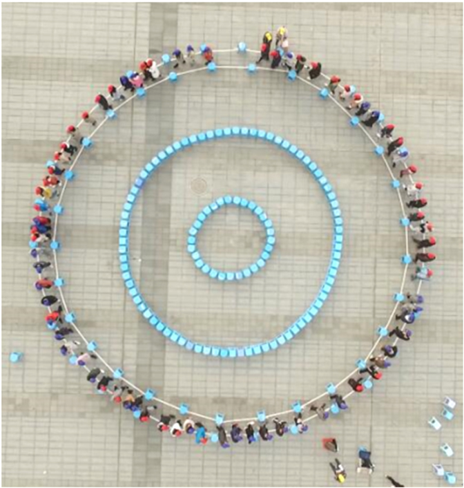
Fig. 1. The basic configuration of the first experiment: one snapshot of Run (6,3).
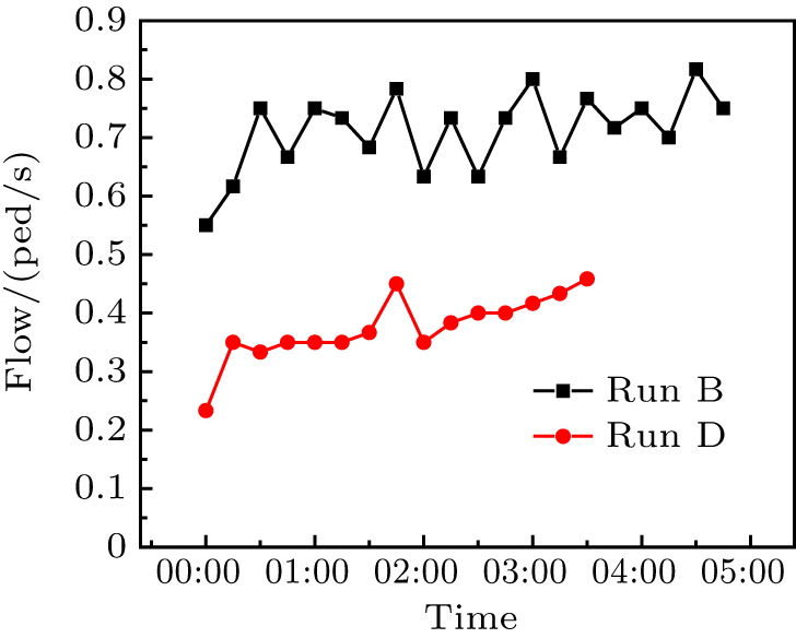
Fig. 2. Averaged flow rates in single-file experiments without bottleneck, including Run B with ρ = 1.5 ped/m and Run D with ρ = 2.5 ped/m.
Fig. 3. Situation with averaged flow rate of 0.33 ped/s for (a) Run (6,2), and (b) Run D when ρ = 2.5 ped/m.
Fig. 4. Angular trajectories of 16 typical pedestrians in runs when the flow rate is 0.33 ped/s of (a) Run (6, 2) and (b) Run D when ρ = 2.5 ped/m.
Fig. 5. Positions of 5 detectors in Run (5, 2).
Fig. 6. The statistics of velocities in runs of the first experiment, when bottleneck is activated for (a) averaged velocities (AV) and (b) standard deviations of velocities (SDV).
Fig. 7. Statistics of time-headways in runs of the first experiment, when bottleneck is activated for (a) averaged time (AT) headways, and (b) standard deviations of time (SDT) headways.
Fig. 8. Basic configuration of the second experiment: (a) snapshot of Run (20, 2) and (b) corresponding route and scales on the ground.
Fig. 9. Trajectories of some typical pedestrians in the second experiment for (a) Run (10, 1), (b) Run (20, 2), (c) Run (10,2), (d) Run (20,4), (e) Run (10,3), and (f) Run (20,6).
Fig. 10. Statistics of all pedestrians’ velocities at different time instants in Run (10, 2).
Fig. 11. Statistics of velocities in 3 runs of the second experiment, when X = 10 s showing (a) averaged velocities, (b) standard deviations of velocities.
Fig. 12. Statistics of time-headways in 3 runs of the second experiment, when X = 10 s, showing (a) averaged time-headways and (b) standard deviations of time-headways.
Fig. 13. Relationships between averaged velocity and corresponding 5-m area in the second experiment.
Fig. 14. Relationships between standard deviation of velocity and corresponding 5-m area in the second experiment.
Fig. 15. PPPM versus time in Run (10, 1) and Run (20, 2) for comparison.
|
Table 1. Details of each run in the first experiment.
|
Table 2. Details of each run in the second experiment.


Set citation alerts for the article
Please enter your email address

© Copyright 2018-2021 | Chinese Laser Press. All Rights Reserved 沪ICP备15018463号-20