Measurement Algorithm for Anti-Stress Cone Parameters of Cross-Linked Polyethylene Cable Joint Based on Three-Dimensional Point Cloud Processing

Lei Deng; Guihua Liu; Hao Deng; Junjie Huang; Binghong Zhou

doi:10.3788/CJL220785

Journals >Chinese Journal of Lasers >Volume 50 >Issue 6 >Page 0604003 > Article

Chinese Journal of Lasers
Vol. 50, Issue 6, 0604003 (2023)

Measurement Algorithm for Anti-Stress Cone Parameters of Cross-Linked Polyethylene Cable Joint Based on Three-Dimensional Point Cloud Processing

Lei Deng^1、2, Guihua Liu^1、2、*, Hao Deng^1、2, Junjie Huang^1、2, and Binghong Zhou^1、2

Author Affiliations

¹School of Information Engineering, Southwest University of Science and Technology, Mianyang 621010, Sichuan, China

²Key Laboratory of Special Environment Robotics of Sichuan Province, Mianyang 621010, Sichuan, China

show less

DOI: 10.3788/CJL220785 Cite this Article Set citation alerts

Lei Deng, Guihua Liu, Hao Deng, Junjie Huang, Binghong Zhou. Measurement Algorithm for Anti-Stress Cone Parameters of Cross-Linked Polyethylene Cable Joint Based on Three-Dimensional Point Cloud Processing[J]. Chinese Journal of Lasers, 2023, 50(6): 0604003 Copy Citation Text

show less

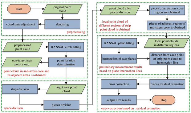
Fig. 1. Flow of anti-stress cone of cable joint parameter measurement algorithm

Download full size

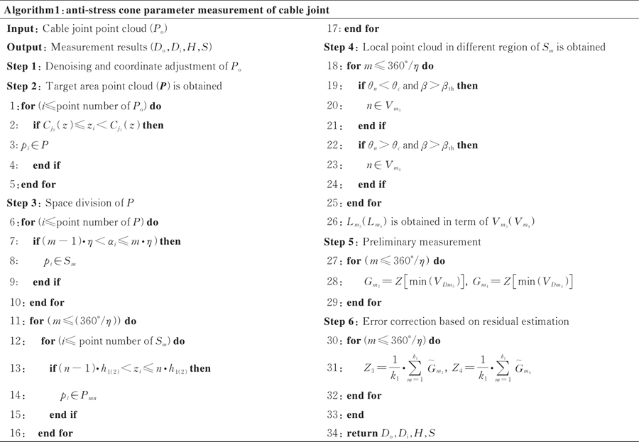
Fig. 2. Pseudocode of anti-stress cone of cable joint parameter measurement algorithm

Download full size

Fig. 3. Cable joint.(a) Structure diagram; (b) physical diagram; (c) point cloud data

Download full size

Fig. 4. Coordinate adjustment diagrams. (a) Before adjustment; (b) after adjustment

Download full size

Fig. 5. Diagram of obtaining target point cloud. (a) Joint point cloud; (b) circle fitting results of joint point cloud; (c) target point cloud fitting circle; (d) target point cloud

Download full size

Fig. 6. Change of cable joint fitting circle radius

Download full size

Fig. 7. Space division of cable joint point cloud.(a) Target point cloud; (b) strips division mode; (c) strips division results of figure (a); (d) an example of strip point cloud; (e) pieces division results of figure (a); (f) an example of piece

Download full size

Fig. 8. Analysis of piece points obtained by different space division methods. (a) Ours; (b) equal height division

Download full size

Fig. 9. Concave-convex decision diagrams. (a) Convex diagram;(b) concave diagram

Download full size

Fig. 10. Change of piece axis angle on strip point cloud

Download full size

Fig. 11. Diagram of strip point cloud formed by planes and surfaces

Download full size

Fig. 12. Calculation process diagram of starting point and ending point of anti-stress cone

Download full size

Fig. 13. Diagram of error correction based on residual estimation

Download full size

Fig. 14. Diagram of measured parameter of anti-stress cone

Download full size

Measuredparameter	Meaning	Calculation method
D_i	End diameter	Diameter of fitting circle at $Z_{4}$
D_o	Start diameter	Diameter of fitting circle at $Z_{3}$
H	Height	$Z_{4} - Z_{3}$
S	Slope length	$\sqrt[]{{[(D_{o} - D_{i}) / 2]}^{2} + H^{2}}$

Table 1. Explanation of measured parameters of anti-stress cone and their calculation methods

Joint	Index	Measured value of radius change				Measured value of ours
Joint	Index	D_i	D_o	S	H	D_i	D_o	S	H
Standard joint	x^* /mm	46.40	78.40	57.28	55.00	46.40	78.40	57.28	55.00
	x /mm	48.35	75.63	49.28	47.35	46.29	78.39	57.42	55.13
	e（x）/mm	-1.95	2.77	8.00	7.65	0.11	0.01	-0.14	-0.13
	e_r（x）/%	4.20	3.53	13.97	13.91	0.24	0.01	0.24	0.24
	Points	766310				766310
	Time /s	6.63				18.87
Artificial joint^①	x^* /mm	47.00	78.00	53.79	51.50	47.00	78.00	53.79	51.50
	x /mm	49.84	76.13	45.62	43.68	46.88	78.32	53.21	50.83
	e（x）/mm	-2.84	1.87	8.17	7.82	0.12	-0.32	0.58	0.67
	e_r（x）/%	6.04	2.40	15.18	15.18	0.26	0.41	1.08	1.30
	Points	814402				814402
	Time /s	7.14				19.85
Artificial joint^②	x^* /mm	45.50	77.50	59.68	57.50	45.50	77.50	59.68	57.50
	x /mm	46.62	74.87	52.69	50.76	45.97	77.21	59.28	57.19
	e（x）/mm	-1.12	2.63	6.99	6.74	-0.47	0.29	0.40	0.31
	e_r（x）/%	2.46	3.39	11.71	11.72	1.03	0.37	0.67	0.54
	Points	898623				898623
	Time /s	7.74				19.38

Table 2. Measurement results of different methods

Joint	Index	Measured value of equal height division				Measured value of ours
Joint	Index	D_i	D_o	S	H	D_i	D_o	S	H
Standard joint	x^* /mm	46.40	78.40	57.28	55.00	46.40	78.40	57.28	55.00
	x /mm	47.16	76.36	55.56	53.60	46.29	78.39	57.42	55.13
	e（x）/mm	-0.76	2.04	1.72	1.40	0.11	0.01	-0.14	-0.13
	e_r（x）/%	1.64	2.60	3.00	2.55	0.24	0.01	0.24	0.24
	Points	766310				766310
	Time /s	18.36				18.87
Artificial joint^①	x^* /mm	47.00	78.00	53.79	51.50	47.00	78.00	53.79	51.50
	x /mm	47.87	76.84	52.66	50.63	46.88	78.32	53.21	50.83
	e（x）/mm	-0.87	1.16	1.13	0.87	0.12	-0.32	0.58	0.67
	e_r（x）/%	1.85	1.49	2.10	1.69	0.26	0.41	1.08	1.30
	Points	814402				814402
	Time/s	19.64				19.85
Artificial joint^②	x^* /mm	45.50	77.50	59.68	57.50	45.50	77.50	59.68	57.50
	x /mm	46.16	76.81	58.92	56.89	45.97	77.21	59.28	57.19
	e（x）/mm	-0.66	0.69	0.76	0.61	-0.47	0.29	0.40	0.31
	e_r（x）/%	1.45	0.89	1.27	1.06	1.03	0.37	0.67	0.54
	Points	898623				898623
	Time /s	19.43				19.38

Table 3. Measurement results for different space division methods

Joint	Index	Measured value before error correction				Measured value after error correction
Joint	Index	D_i	D_o	S	H	D_i	D_o	S	H
Standard joint	x^* /mm	46.40	78.40	57.28	55.00	46.40	78.40	57.28	55.00
	x /mm	46.29	78.39	57.42	55.13	46.29	78.39	57.42	55.13
	e（x）/mm	0.11	0.01	-0.14	-0.13	0.11	0.01	-0.14	-0.13
	e_r（x）/%	0.24	0.01	0.24	0.24	0.24	0.01	0.24	0.24
	Points	766310
	Time /s	18.87
Artificial joint^①	x^* /mm	47.00	78.00	53.79	51.50	47.00	78.00	53.79	51.50
	x /mm	47.46	77.36	51.45	49.23	46.88	78.32	53.21	50.83
	e（x）/mm	-0.46	0.64	2.34	2.27	0.12	-0.32	0.58	0.67
	e_r（x）/%	0.98	0.82	4.35	4.41	0.26	0.41	1.08	1.30
	Points	814402
	Time /s	19.85
Artificial joint^②	x^* /mm	45.50	77.50	59.68	57.50	45.50	77.50	59.68	57.50
	x /mm	46.36	76.06	57.12	55.16	45.97	77.21	59.28	57.19
	e（x）/mm	-0.86	1.44	2.56	2.34	-0.47	0.29	0.40	0.31
	e_r（x）/%	1.89	1.85	4.29	4.07	1.03	0.37	0.67	0.54
	Points	898623
	Time /s	19.38

Table 4. Measurement results before and after error correction

h /mm	H /mm	e（x）/mm	e_r（x）/%
0.1	55.61	-0.61	1.11
0.2	55.52	-0.52	0.95
0.3	55.43	-0.43	0.78
0.4	55.38	-0.38	0.69
0.5	55.25	-0.25	0.45
0.6	55.53	-0.53	0.96
0.7	55.74	-0.74	1.35
0.8	55.87	-0.87	1.58
0.9	56.01	-1.01	1.84
1.0	56.12	-1.12	2.04

Table 5. Effect of piece height h on algorithm accuracy

η /（°）	H /mm	e（x）/mm	e_r（x）/%
1	61.07	-3.57	6.21
2	60.17	-2.67	4.64
3	59.37	-1.87	3.25
4	58.40	-0.90	1.57
5	57.96	-0.46	0.80
6	57.18	0.32	0.56
7	56.62	0.88	1.53
8	56.13	1.37	2.38
9	55.47	2.03	3.53
10	54.10	3.40	5.91

Table 6. Effect of strip point cloud angle η on algorithm accuracy

D_th3	H /mm	e（x）/mm	e_r（x）/%
0.10	60.75	-3.25	5.65
0.15	59.83	-2.33	4.05
0.20	59.34	-1.84	3.20
0.25	58.63	-1.13	1.97
0.30	58.14	-0.64	1.11
0.35	57.96	-0.46	0.80
0.40	57.13	0.37	0.64
0.45	56.73	0.77	1.34
0.50	56.31	1.19	2.07
0.55	55.81	1.69	2.94

Table 7. Effect of threshold D_th3on algorithm accuracy

D_th4	H /mm	e（x）/mm	e_r（x）/%
0.10	61.03	-3.53	6.14
0.15	60.47	-2.97	5.17
0.20	59.67	-2.17	3.77
0.25	59.14	-1.64	2.85
0.30	58.66	-1.16	2.02
0.35	57.96	-0.46	0.80
0.40	57.36	0.14	0.24
0.45	56.78	0.72	1.30
0.50	56.21	1.29	2.24
0.55	55.73	1.77	3.08

Table 8. Effect of threshold D_th4on algorithm accuracy

Download Citation

Set citation alerts for the article

Tools

Set citation alerts for the article

Save the article for my favorites

Paper Information