
Jinglin Zhao, Zhiqiang Wang, Jinjun Wang, Dongdong Zhang, Guofeng Li. Deposited energy optimization analysis of discharge in water based on Kriging model[J]. High Power Laser and Particle Beams, 2023, 35(3): 035005
- High Power Laser and Particle Beams
- Vol. 35, Issue 3, 035005 (2023)
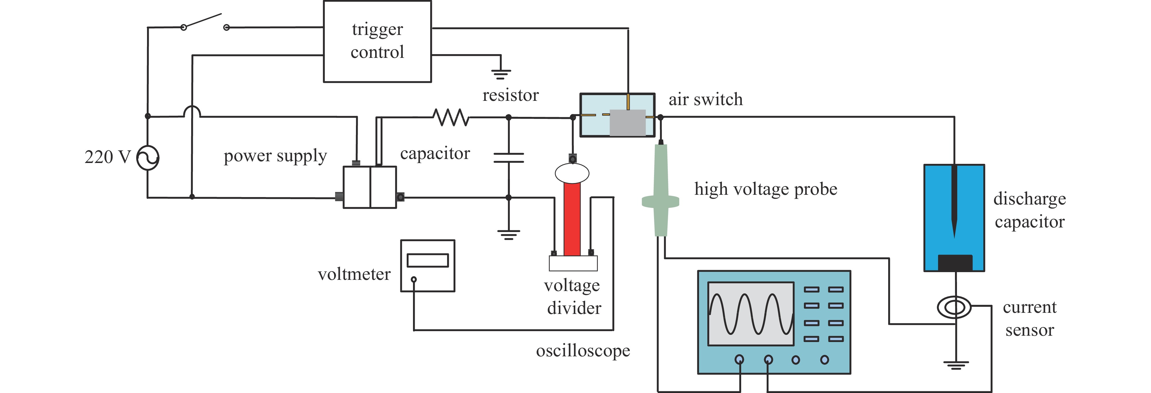
Fig. 1. Schematic diagram of underwater high-voltage pulse discharge experiment system
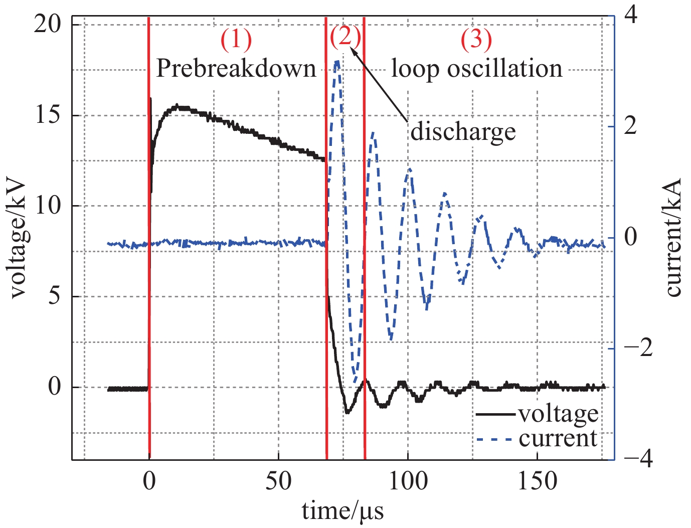
Fig. 2. Typical voltage and current waveform of high voltage pulse discharge in water
Fig. 3. Plasma channel development process
Fig. 4. Results of deposited energy calculation
Fig. 5. Flowchart of the optimization search analysis
Fig. 6. Spatial distribution of the 20 initial sample points
Fig. 7. Cross-validation of the computational process
Fig. 8. Variation of root mean square error with the number of additions
Fig. 9. Multi-peak characteristics of deposited energy
Fig. 10. Global optimization search flow chart
Fig. 11. Comparison between experimental results and optimal deposited energy
|
Table 1. Experimental variables and their scope
|
Table 2. Some of the initial sample points after inverse normalization and the corresponding experimental results
|
Table 3. After the normalization of some of the new points and the corresponding experimental results
|
Table 4. Effect of electrode spacing variation on deposited energy at different conductivities
|
Table 5. Global optimal solution of the model


Set citation alerts for the article
Please enter your email address

© Copyright 2018-2021 | Chinese Laser Press. All Rights Reserved 沪ICP备15018463号-20