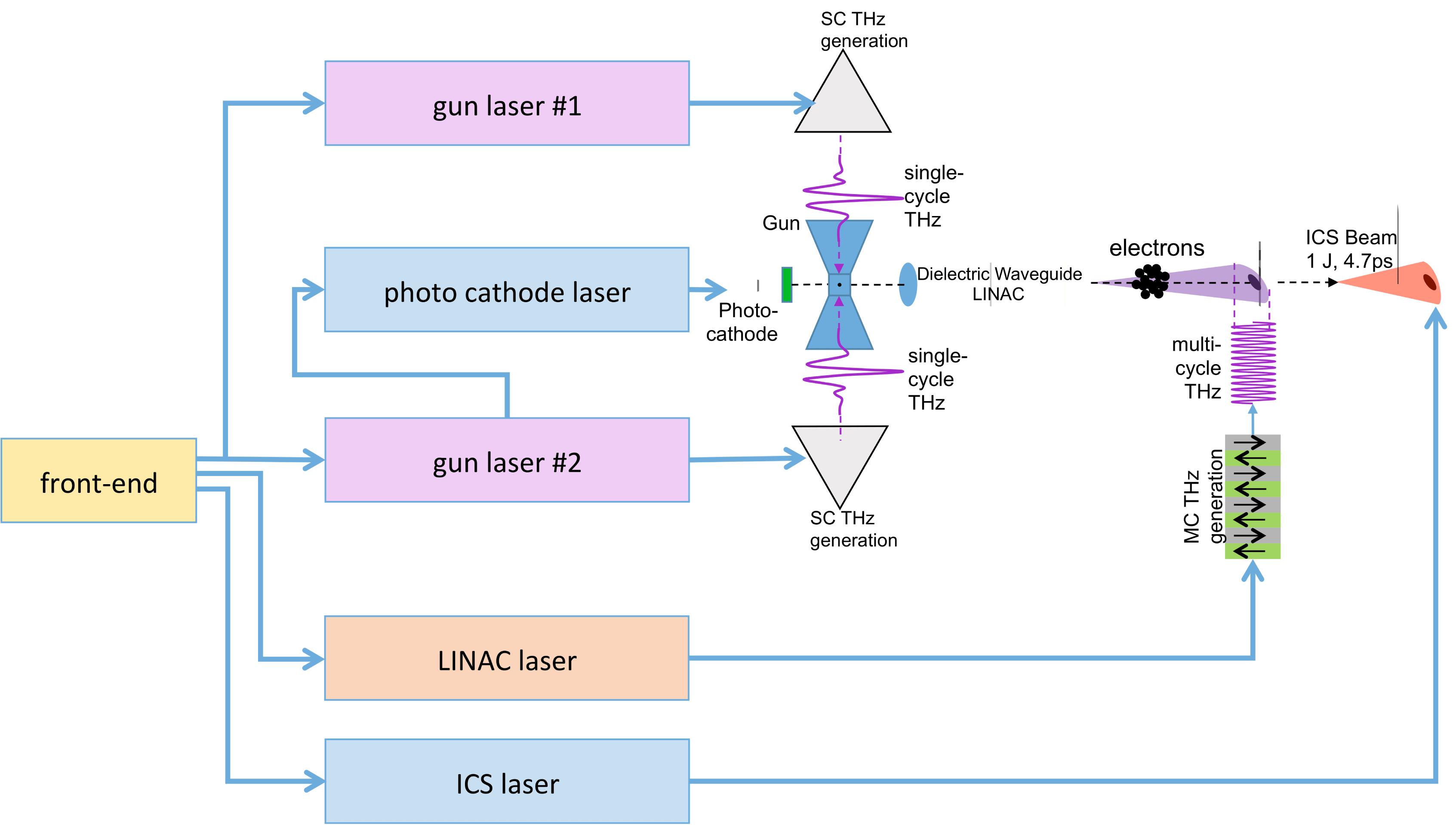
Fig. 1. Schematic representation of the THz-driven light source with the driving laser system. SC: single-cycle; MC: multi-cycle, ICS: inverse Compton scattering.

Fig. 2. Computed amplified spectral bandwidth as a function of seed energy in a Yb:YAG thin-disk regenerative amplifier ($\unicode[STIX]{x0394}\unicode[STIX]{x03BB}_{\text{Fluo}}=5$ nm).

Fig. 3. The cryogenic composite thin disk: in our approach, a thin Yb:YAG gain sheet is diffusion bonded to a thicker index-matched cap on one face while the other face is HR coated and soldered to a backplane high-performance cooler. See text for details.

Fig. 4. Photographs of the (a) 100 mJ and (b) 1 J Yb:YAG amplifier.

Fig. 5. (a) Measured output spectrum (black line) at the 10 mJ energy level along with seed spectrum (grey shaded region). (b) Measured output energy versus pump input fluence characteristics showing an output energy ${\sim}$90 mJ at full pump power.

Fig. 6. CAD modeling of (a) the grating compressor currently in use after a Yb:YAG high-energy amplifier and (b) the holder of the large grating in the first compressor built in our lab after the Yb:KYW regenerative amplifier^[47]. (c) A newer version of the grating holder, implemented for the Yb:YLF laser system.

Fig. 7. Schematic of the two-stage OPA system to drive the UV generation setup. In the prism compressor located between the two OPA stages, a pulse shaper is implemented: knifes block the highest and lowest spectral components. WL: white-light generation, SHG: second harmonic generation, Comp: compressor.

Fig. 8. (a) Spectra of the first and second OPA stages (OPA1 and OPA2). (b) Autocorrelation trace of the second OPA stage after the prism compressor and the corresponding Gaussian fit.

Fig. 9. (a) Simultaneous measurement of the energy at the output of the Yb:KYW regenerative amplifier, pointing measured after the regenerative amplifier, and stretched spectrum. Only a fraction of the energy of the regenerative amplifier is measured without rescaling to the total energy. An rms value for the relative energy fluctuations of 0.8% is measured. The stretched spectrum was measured with a 12.5 GHz photodiode and a 4 GHz oscilloscope. (b) Long term measurement of the Yb:KYW regenerative amplifier output.

Fig. 10. (a) Measured 1-h stability of the regenerative amplifier output at the 10 mJ energy level. The computed shot-to-shot instabilities are less than $\pm 0.75\%$ rms over 1-h. In inset, the measured spatial intensity profile at 10 mJ output energy. (b) Measured output energy stability recorded over 3.5 h at ${\sim}$75 mJ output energy. The observable slow drift is attributed to a minor drift in seed energy of the current frontend. Energy instabilities less than $\pm 0.7\%$ over 3.2 h are routinely achieved.

Fig. 11. Pulse energy measurement of the compressed OPA output over 15 h.

Fig. 12. Schematic representation of the laser system based on cryo-Yb:YAG laser systems.

Fig. 13. Schematic representation of the laser system based on cryo-Yb:YLF and cryo-Yb:YAG laser systems.

Fig. 14. Schematic representation of the laser system based on RT-Yb:YAG laser systems.

Fig. 15. Layout of two Yb:YAG laser chains on one optical table. The seed pulses are fiber delivered. The delay stage (dt) is followed by the Yb:KYW regenerative amplifier (REG), followed by the two CTD amplifiers with a relay imaging telescope (R.Tel) in between. After the regenerative amplifier and the first CTD amplifier, there is a pointing stabilizer. The spatial profile of the beam is measured after each stage. The alignment laser for first alignment of the 100 mJ CTD is represented.

Table 1. Summary of the requirements of each laser chain. The THz energy takes into account the transport losses (for single-cycle THz pulses, twice the required energy within the gun is accounted for, and ${\sim}1.5$ for multi-cycle THz pulses).

Table 2. Summary of the spectroscopic and thermo-optic properties of Yb:YAG at RT and CT and Yb:YLF at cryogenic temperature.

Table 3. Description of the main outputs of the frontend.

Table 4. Summary of the pulse parameters after each module of the CT Yb:YAG laser chain.

Table 5. Summary of the pulse parameters after each module of the RT-Yb:YAG laser chain.

Table 6. Summary of the pulse parameters after each module of the CT-Yb:YLF laser chain.

Table 7. Diagnostics for the modules.