
Ping Zhu, Xinglong Xie, Xiaoping Ouyang, and Jianqiang Zhu, "Output temporal contrast simulation of a large aperture high power short pulse laser system," High Power Laser Sci. Eng. 2, 04000e42 (2014)
- High Power Laser Science and Engineering
- Vol. 2, Issue 4, 04000e42 (2014)
Abstract
1. Introduction
With the development of chirped-pulse amplification (CPA) and optical parametric CPA (OPCPA), extremely intense short pulse laser systems are increasingly applied to experimental investigations in ‘fast ignition’ inertial confinement fusion (ICF), laser–plasma interactions and strong field physics[ single laser beamline (ILE)[
High energy laser systems usually enlarge the beam diameter to reduce the energy density on optical elements to mitigate the limited damage threshold problem, which inevitably leads to worse near-field quality, such as near-field intensity modulation and wavefront deviation. Means have existed for some time to analyze the influence on spatial output characteristics by wavefront deviation[
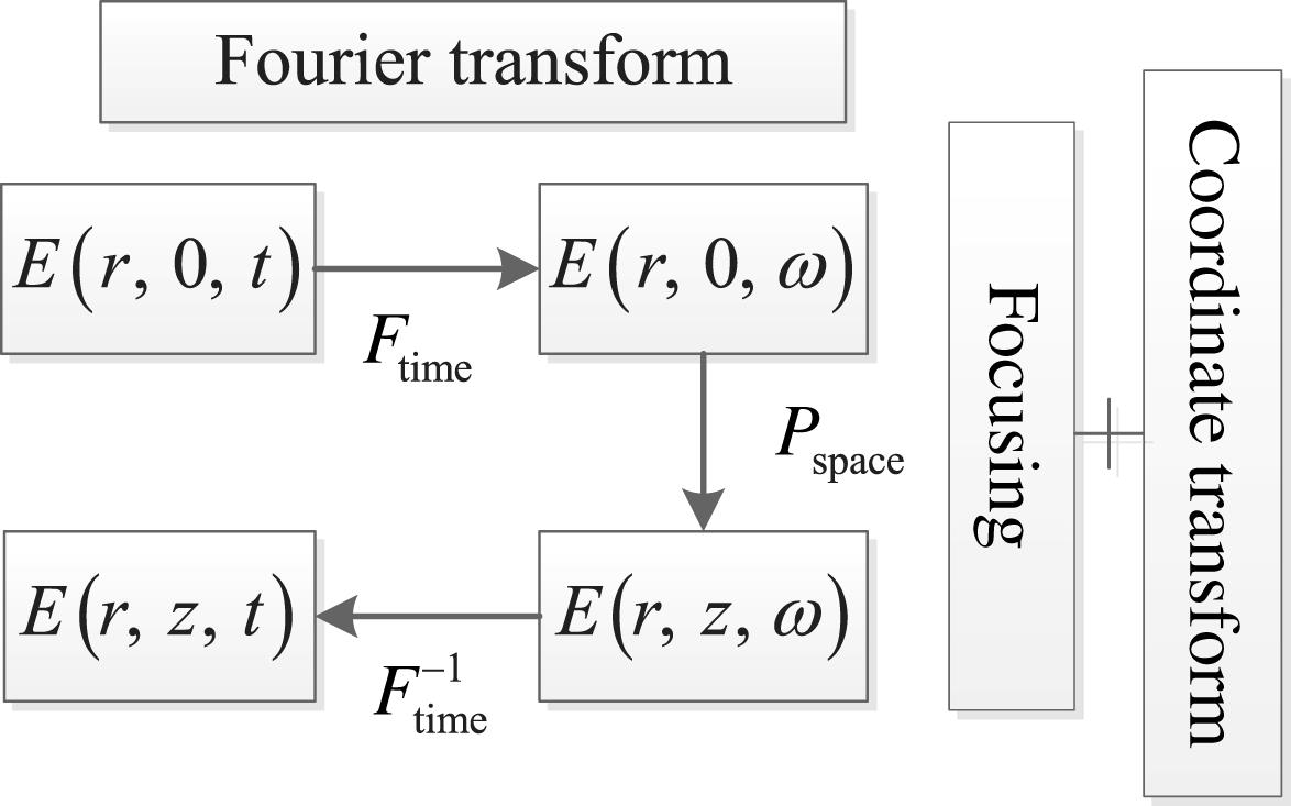
In large aperture high power short pulse laser systems, the output is focused by an off-axis parabolic mirror (OAP), and this focusing propagation can be well simulated by a two-step coordinate transformed focusing method, not only taking advantage of using coordinate transformation but also avoiding the contradiction between the space scale and the diffraction limit[
Sign up for High Power Laser Science and Engineering TOC. Get the latest issue of High Power Laser Science and Engineering delivered right to you!Sign up now
2. Theory and simulation
2.1. Model
In practical short pulse applications, the amplified pulse by CPA or OPCPA will be focused onto the target using an OAP after being compressed by a grating compressor. The analogy can be made between the OAP focusing subsystem and an ideal lens, because it linearly reflects propagation in free space without dispersion, chromatic aberration or B-integral nonlinear effects, the spatial intensity distribution of which can be calculated by the Fresnel diffraction integral formula:
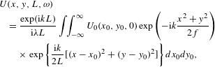 (1)
(1) and
and  are the coordinates in the observation plane
  ,
,  and
and  are the coordinates in the incident plane,
  is the wavelength of the incident pulse,
  is the wavevector and
  is the focal length of the OAP.
For higher spatial resolution and a more accurate result, on applying the coordinate transforms  ,
,  and
and  , Equation (
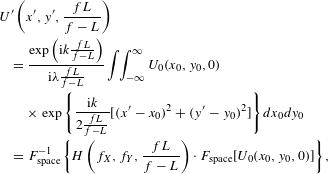 (2)
(2) (3)
(3) and
and  are the spatial frequencies in the
  and
and  directions, respectively, and the spatial Fourier transform and its inverse form are introduced to reduce the computing time by the fast Fourier transform (FFT) algorithm:
 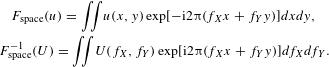 (4)
(4)When Equation ( ), a problem of infinite
  ,
,  and
and  is encountered, which can be ingeniously resolved by a two-step simulation, first calculating from
  to
to  with coordinate transforms and finally calculating from
  to
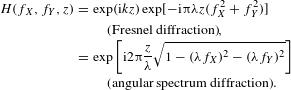
to  without coordinate transforms, in which angular spectrum diffraction theory is applied. The value of
  is related to the coordinate magnification, which determines whether there are sufficient effective sampling points in the focal spot area. At the same time, the value of
  determines whether the situation meets the requirement for the Fresnel approximation in step one with coordinate transforms. With this method in two spatial dimensions, the calculation of the focusing characteristics of a short wavelength laser beam through a short focus system has been successfully made[
Thus, we can use an operator  to represent the above focusing calculation:
 (5)
(5)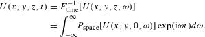 (6)
(6)2.2. Near-field intensity modulation
In large aperture high power laser systems, light beams are always shaped into flattened Gaussian beams (FGBs) for higher energy extraction efficiency and slower nonlinear growth. A FGB of order  and spot size
  has the following normalized field distribution[
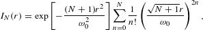 (7)
(7) is the radial coordinate.
In practical applications, the real near-field intensity is always modulated rather than an ideal FGB due to multiple causes, such as diffraction and nonlinear growth. The fill factor (FF) of the laser beam is usually used to describe the uniformity of the modulated near-field intensity, which is defined as the ratio of the average intensity and the peak intensity in the flattened area:
 (8)
(8)2.3. Wavefront deviation
The ideal incident wavefront is plane; however, it can be easily deviated by phase shifts from the optical system and optical elements. Phase shifts from the optical system, such as thermal deformation and inhomogeneity of the medium, mainly contribute to dynamic wavefront deviation on a large spatial scale, which can be detected online by a Shack–Hartmann wavefront sensor. According to research carried out at Lawrence Livermore National Laboratory[ ), waviness (
 ) and roughness (higher than
  ), which can be expressed by the improved noise model[
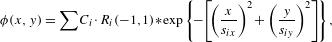 (9)
(9) is the noise magnitude,
  is a random function distributed between
  and 1,
  represents a convolution operation,
  and
and  are the spatial scales in the
  and
and  directions, respectively, determining the noise spatial length. The total wavefront deviation is the sum of noise of every spatial length. Common evaluation indices of wavefront deviation are the peak to valley (PV) value, root mean square (RMS), RMS gradient (GRMS) and power spectral density (PSD) curve.
3. Results and discussion
The parameters of the analyzed large aperture high power short pulse model are those of the SG-II laser system[ to 160 mm and 2048 points in time from
  to 100 ps. The value of
  is the key parameter of the simulation due to the two reasons mentioned above. Here, we use
  to reach the requirements of both high resolution and the Fresnel approximation, then we obtain the convergence results.
3.1. Temporal contrast degradation by intensity modulation
First, the influence of intensity modulation on temporal contrast is analyzed. The model applied here is a ninth-order FGB with a diameter of 290 mm, and its near-field intensity is modulated randomly in three situations for which the FFs are 0.4, 0.6 and 0.8, respectively, as shown in Figure
Figure  (blue dashed line). A pre-pulse can be seen 50 ps before the main pulse when the near-field intensity is modulated, which leads to a poor temporal contrast. Moreover, the front edge of the main pulse becomes moderate 10–20 ps ahead of the peak point, which means that the pulse width of the main pulse will be broadened at the same time. When the intensity is modulated by a FF of 0.6, the temporal contrast will be degraded by more than one order of magnitude to worse than
  in the time window of 50 ps before the main pulse. The tendency can be seen from this figure that the smaller the FF of the modulated intensity is the worse the output temporal contrast is.
3.2. Temporal contrast degradation by wavefront deviation
Second, using the same model as described above, the effect of wavefront deviation on temporal contrast is discussed. At this time the incident intensity has no modulation, but various types of random wavefront deviations are introduced in the focusing propagation, which have different magnitudes and different spatial frequencies. As shown in Figure
Figure  . Comparing the blue line
  with the green line
  in the same spatial frequency range (the same minimum spatial period
  is 40 mm, which means that the same maximum spatial frequency is
  ), the wavefront deviation with larger PV value will cause more severe temporal contrast degradation and in this spatial frequency range the temporal contrast will be two orders of magnitude worse than that of the ideal situation.
When the wavefront deviations have the same magnitude  but different spatial frequency ranges, as shown in Figure
  (cyan line; minimum spatial period of 0.15625 mm) causes huge degradation of more than five orders of magnitude from
  to
to  , while the wavefront deviation with the lowest maximum spatial frequency of
  (green line; minimum spatial period of 40 mm) induces smaller degradation of one order. Interestingly, temporal contrast degradation by the wavefront deviation with the middle maximum spatial frequency of
  (red line; minimum spatial period of 0.625 mm) is quite notable within 40 ps before the main pulse; however, it becomes less significant beyond 40 ps before the main pulse. Therefore, higher spatial frequency contributes to temporal contrast degradation in a larger time window and for the same magnitude the wavefront deviation with low maximum spatial frequency has a slight influence on temporal contrast.
3.3. Influence of diameter on temporal contrast degradation
Third, the importance of discussing temporal contrast in a system with large diameter is demonstrated by analyzing the influence of diameter on temporal contrast degradation. In this case, introducing the same magnitude and same spatial frequency wavefront deviation as shown in Figures
The result can be seen in Figure  in the model with 320 mm diameter without any near-field quality deterioration (cyan dashed line). However, for an ideal thin beam that does not need to be focused, the temporal contrast will be promoted to the computer simulation resolution limit, about
  (purple dotted line). Therefore, temporal contrast degradation deserves more attention in larger aperture high power short pulse laser systems.
3.4. Simulation of temporal contrast degradation compared with experimental measurement results
Finally, the simulation model is combined with the near-field quality measured in the established SG-II large aperture high power short pulse laser system. Figure  , while the calculation result shows a temporal contrast degradation of less than two orders of magnitude from
  . There are two reasons why the two results differ. (1) In this model beam quality is considered as the only influencing factor; however, in real experiments there are many other characteristics, such as ASE, PF and spectral modulation. (2) Only near-field intensity and low spatial frequency wavefront deviation are introduced, without considering waviness and roughness.
To introduce the waviness and roughness into the simulation model, an assumption is made based on the SG-II short pulse laser system configuration. In consideration of the cutoff frequency of the spatial filter, a wavefront deviation of waviness and roughness whose maximum spatial frequency is  is added, as shown in Figure
  , the RMS is
  , the GRMS is
  and the PSD curve is shown in Figure
4. Conclusion
In this paper, a two-step coordinate transformed focusing method is used to simulate the output focused by an OAP in a large aperture high power short pulse laser system, and thus the output temporal contrast is calculated. The temporal contrast degradation by intensity modulation and wavefront deviation is analyzed. It is found that intensity modulation with a smaller FF and larger wavefront deviation causes more severe temporal contrast degradation, and this degradation is closely related to the spatial frequency of the total wavefront deviation. Then, the importance of discussing temporal contrast in a system with large diameter is demonstrated by analyzing the influence of diameter on temporal contrast degradation. Finally, with experimental intensity modulation, experimental low spatial frequency wavefront deviation and assumed higher spatial frequency wavefront deviation using the parameters of the SG-II laser system, the output temporal contrast is derived, which shows that waviness and roughness influence the temporal contrast more seriously. Therefore, the conclusion can be drawn that near-field quality deterioration might lead to temporal contrast degradation, hindering higher temporal contrast in large aperture high power short pulse laser systems.
Due to the lack of effective tools to measure intermediate and higher spatial frequency wavefront deviation, the need for online monitoring of the wavefront deviation in these frequency regions in large aperture high power short pulse laser systems is put forward. Improvement of the laser near-field quality might be a new method towards high temporal contrast in large aperture high power short pulse laser systems.
References
[2] J.-P. Chambaret, F. Canova, R. L. Martens, G. Cheriaux, G. Mourou, A. Cotel, C. Le Blanc, F. Druon, P. Georges, N. Forget, F. Ple, M. Pittman. Proceedings of CLEO/Quantum Electronics and Laser Science Conference and Photonic Applications Systems Technologies JWC4(2007).
[4] C. Li, Z. Zhang, Z. Xu. Acta Opt. Sin., 16, 299(1996).
[6] M. Kalashnikov, A. Andreev, H. Schönnagel. Proc. SPIE, 7501, 750104(2009).
[7] M. P. Kalashnikov, E. Risse, H. Schönnagel, W. Sandner. Opt. Lett., 30, 923(2005).
[9] J. Wang, P. Yuan, J. Ma, Y. Wang, G. Xie, L. Qian. Opt. Express, 21, 15580(2013).
[10] C. Manzoni, J. Moses, F. X. Kärtner, G. Cerullo. Opt. Express, 19, 8357(2011).
[11] A. Guo, H. Zhu, Z. Yang. Acta Opt. Sin., 33(2013).
[12] Q. Liu, Z. Cen, X. Li. Acta Opt. Sin., 33(2013).
[13] M. Yang, M. Zhong, G. Ren. Acta Opt. Sin., 31(2011).
[15] C. R. Wolfe, J. K. Lawson. Proc. SPIE, 2633, 361(1995).
[16] J. K. Lawson, J. M. Auerbach, R. E. English. Proc. SPIE, 3492, 336(1999).
[17] Y. H. Chen, W. G. Zheng, W. J. Chen, S. B. He, J. Q. Su, Y. B. Chen, J. Yuan. High Power Laser Part. Beams, 17, 403(2005).
[18] G. Xu, T. Wang, Z. Li, Y. Dai, Z. Lin, Y. Gu, J. Zhu. Rev. Laser Eng., 36, 1172(2008).
[19] Y. Wang, X. Ouyang, J. Ma, P. Yuan, G. Xu, L. Qian. Chin. Phys. Lett., 30(2013).


Set citation alerts for the article
Please enter your email address

© Copyright 2018-2021 | Chinese Laser Press. All Rights Reserved 沪ICP备15018463号-20