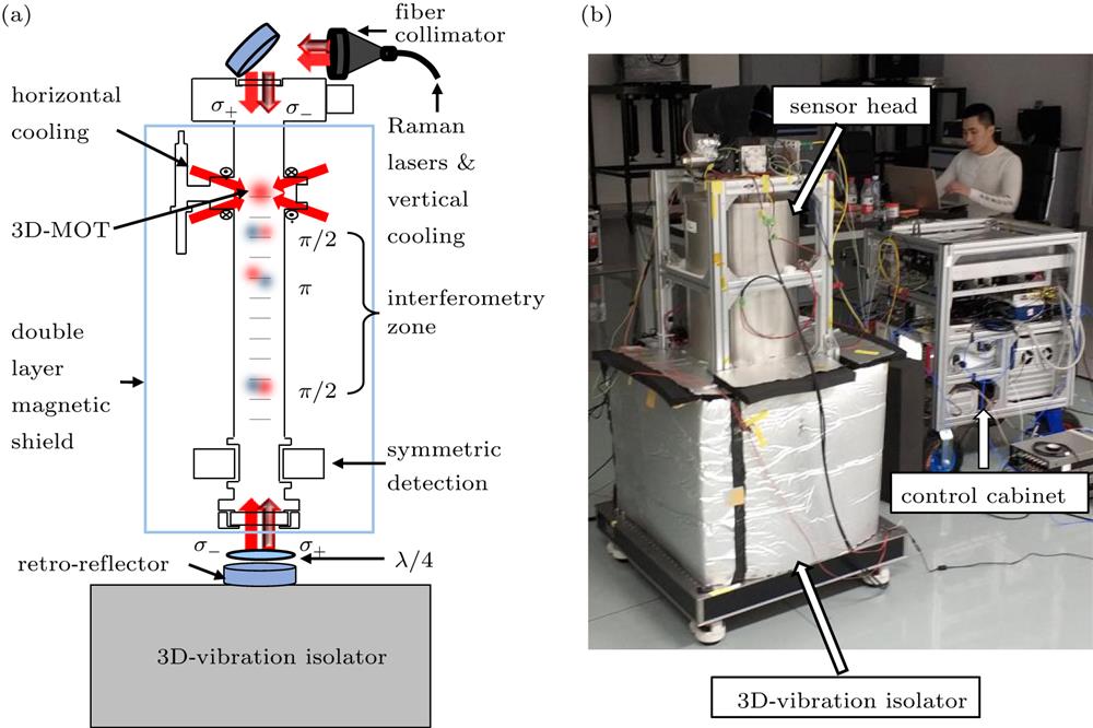
Fig. 1. (a) The schematic diagram of the sensor head of the compact atomic gravimeter USTC-AG02. (b) The photo of USTC-AG02 performing gravity measurement in NIM. It consist of a compact sensor head, a 3D vibration isolator, and a controller.

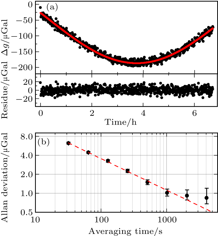
Fig. 2. Continuous g measurement at NIM, started from 2019-01-20T12:17Z. (a) Top: the black points indicate the g measurement data. Each datum is an average of 96 drops (32 seconds). The red curve indicates the Earth’s tide. Bottom: the residues between the measurement data and the Earth’s tide. (b) The black points and bars indicate the Allan deviations of the residues. The red line indicates the average expected for white noise.

Fig. 3. Continuous g measurement at NIM, started from 2019-01-20T12:17Z. (a) The diagram of the two pairs of Raman beams. If the chirp rate is –α_u (+α_d), then k_eff > 0 (k_eff < 0). (b) Interferometry fringes for the two configurations of k_eff. Each of them is obtained by 48 drops in 16 s for chirping up or down. Each black dot is the probability of the atoms in |1,0〉 state by averaging of 4 drops. The error bars represent the statistical errors. The purple (red) line is the fitting curve according to the chirp rate of –α_u (+ α_d). (c) Allan deviations of the gravity signal corrected for Earth’s tides, in the k_eff > 0 (purple) configuration and the k_eff < 0 (red) configuration, respectively. The dashed lines indicate the averaging expected for white noise.

Fig. 4. Variation of the shift of the measured g value due to the TPLS versus the Rabi frequency ratio. Each g value is an average of about 30 minutes. The ratio of 1.0 corresponds to 2π × 25.7 kHz. The red line is a linear fit of the data.

Fig. 5. (a) The schematic of the Coriolis force related to the Earth’s rotation. Left: The Earth’s top view above the north pole. Right: The Earth’s side view parallel to the equator. The blue (or red) arrows represent the horizontal velocity direction v_W (or v_E) of the atom cloud and the corresponding Coriolis force direction. (b) Measured g values for two opposite orientations of the sensor head (0° and 180°).

Fig. 6. (a) The figure of the SAE analysis for the entirety of USTC-AG02. We set the 3D-MOT center as z = 0. The 4 dashed lines (z = A, B, C, D) represent the atoms center positions at the 3 Raman pulses. The red dots indicate the gravitational acceleration in z direction along the atomic trajectory; the blue line indicates the integration of Γ over z. (b) The SAE contributions of USTC-AG02’s all components.

Fig. 7. The calculated influence of the gravity gradient (T_zz ≈ 300 μGal/m) near the surface of the Earth. The red line indicates the perturbation along the atomic trajectory; the blue line indicates the integration of the perturbation over z. The result is independent of T_zz, but for the sake of convenience.

Table 1. The noise budget of USTC-AG02.

Table 2. Systematic errors of the device and the environmental effects budget. The bias of the environmental effects is at the moment of 2019-01-16T16:00Z, in NIM.