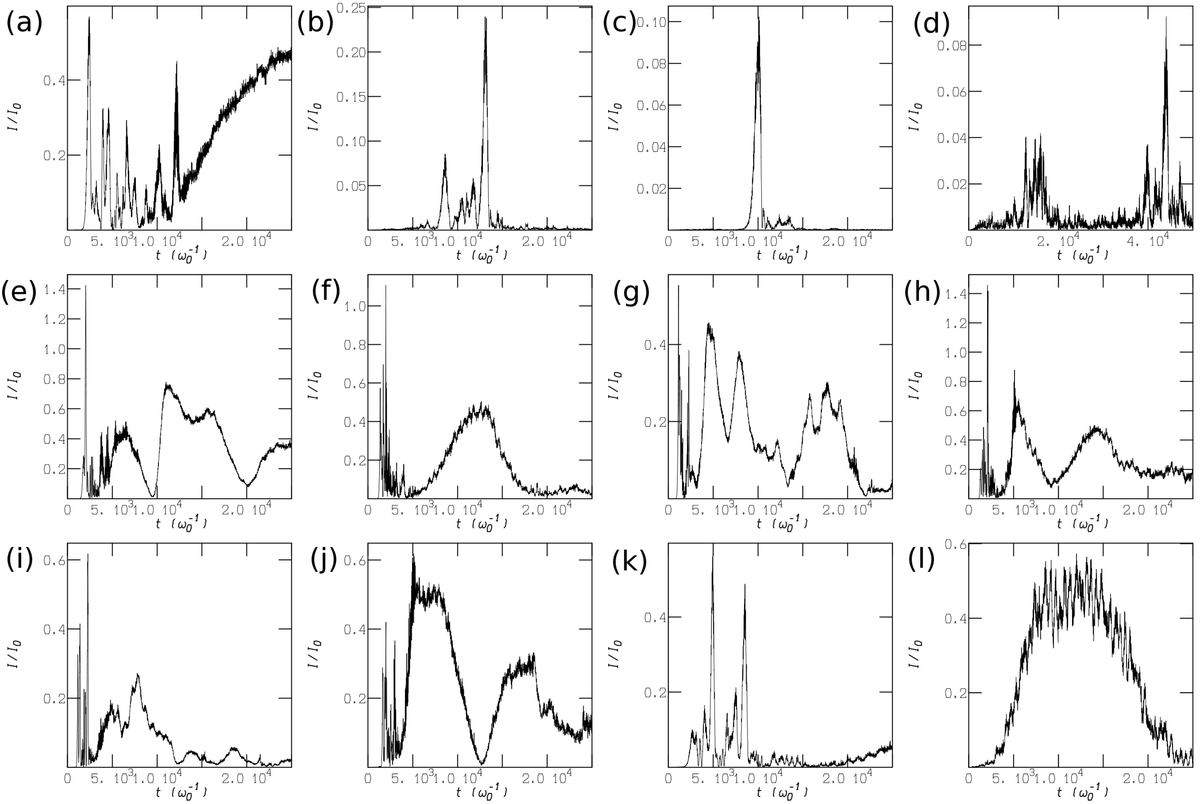
Fig. 1. Reflectivity evolution: backscattered intensity normalized to incident intensity. The subfigures correspond to the following cases in Table 1: I (a), II (b), IIa (c), IIb (d), III (e), IV (f), IVa (g), V (h), Va (i), VI (j), VII (k), and VIII (l). The index a indicates that the plasma length was reduced to $40~{\rm\mu}\text{m}$, the index b to a doubling of the simulation time (i.e., 25 ps at half the number of particles per computational cell). N.B. reflectivity scales are not the same.

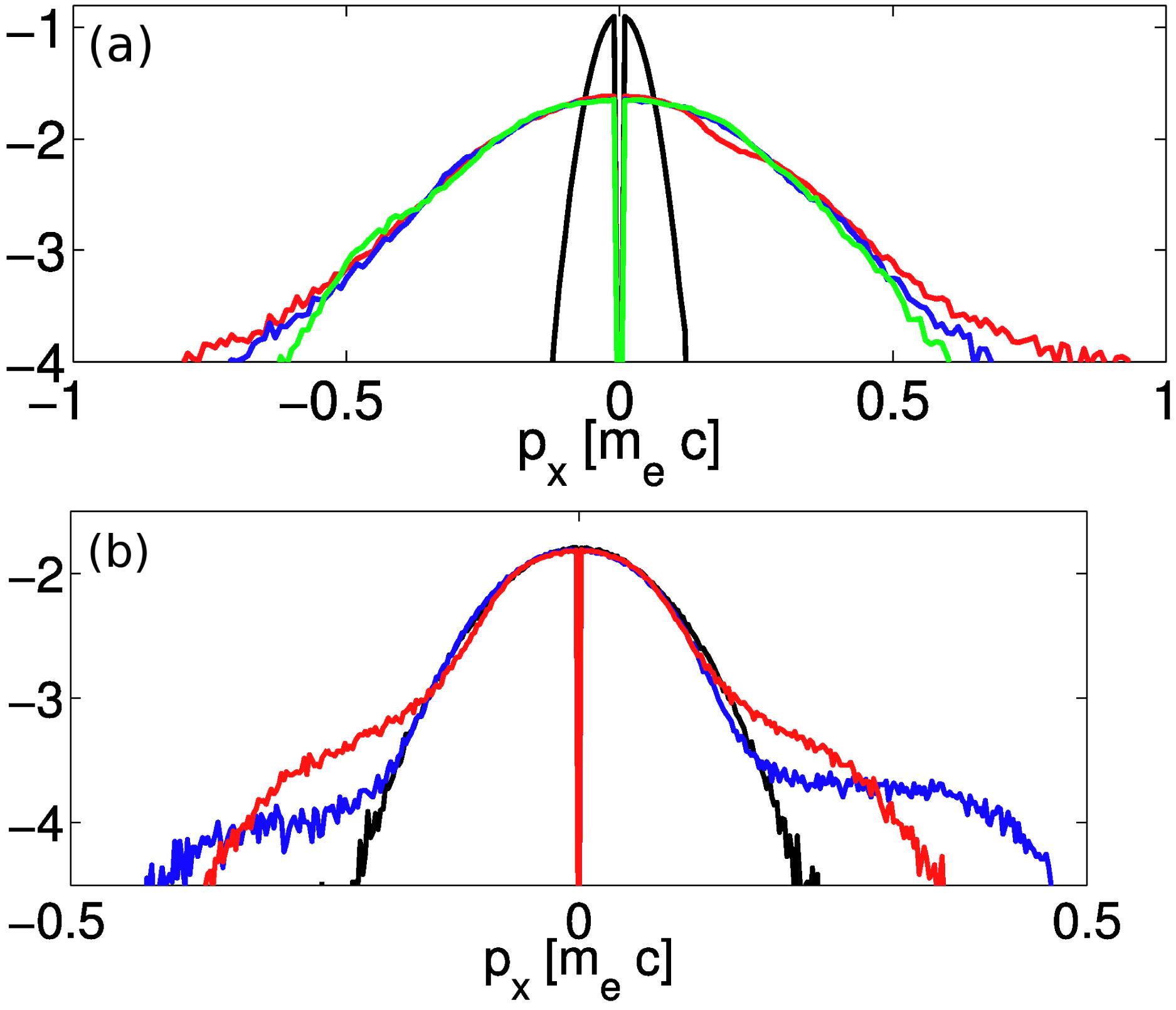
Fig. 2. Parallel electron distribution functions. (a) Case IV for the times: $t=0$ (black), $(0.5\times 10^{4}){\it\omega}_{o}^{-1}$ (red), $(1.1\times 10^{4}){\it\omega}_{o}^{-1}$ (blue) and $(2\times 10^{4}){\it\omega}_{o}^{-1}$ (green). (b) Case VII for the times: $t=0$ (black), $(0.5\times 10^{4}){\it\omega}_{o}^{-1}$ (blue) and $(1\times 10^{4}){\it\omega}_{o}^{-1}$ (red).

Fig. 3. Reflectivity evolution showing the effect of ion mass and electron temperature $T_{e}$ variation. First row with ion mass $1836$ with 1 keV (a), 2 keV (b), 4 keV (c), 8 keV (d). These cases correspond to the following runs in Table 1: (a) – I, (b) – VII, (c) – II, and (d) – X. Second row with ion mass $10^{4}$ with 1 keV (e), 2 keV (f), 4 keV (g), 8 keV (h). Third row with ion mass $10^{5}$ with 1 keV (i), 2 keV (j), 4 keV (k), 8 keV (l). All the simulations used a plasma of $80~{\rm\mu}\text{m}$. The 6 keV cases (not shown here) as function of the three mass ratios show reflectivities on the same level as the 8 keV cases. For all cases $I{\it\lambda}^{2}=10^{15}~\text{W}/\text{cm}^{2}$. Note: scales are not the same.

Fig. 4. Electron distribution functions for the case VII. (a) Snapshots averaged over the whole plasma slab. (b) Time resolved for a plasma slice of width $68c/{\it\omega}_{o}$ located roughly in the middle of the plateau.

Fig. 5. Logarithm of the frequency spectra (case VII) for backscattered light (a) and transmitted light (b). (a) The peaks 1 ($0.336{\it\omega}_{o}$), 2 ($0.658{\it\omega}_{o}$), 3 ($1.0{\it\omega}_{o}$) and 4 ($1.378{\it\omega}_{o}$) correspond to rescatter, RBS-Stokes, laser and RBS-anti-Stokes, respectively. (b) The peaks 1 ($0.332{\it\omega}_{o}$), 2 ($0.682{\it\omega}_{o}$), 3 ($1.0{\it\omega}_{o}$) and 4 ($1.319{\it\omega}_{o}$) correspond to rescatter, RFS-Stokes, laser and RFS-anti-Stokes, respectively.

Fig. 6. Logarithm of the $k$-spectrum of the transverse electric field at $t=(5.5\times 10^{3}){\it\omega}_{o}^{-1}$ (case VII) showing the principal decay as well as the secondary decay of the electromagnetic wave. The spectrum comprises the whole computational box, i.e., plasma, left vacuum and right vacuum. The peaks are located at: $0.11k_{o}$ (1), $0.34k_{o}$ (2), $0.59k_{o}$ (3), $0.67k_{o}$ (4), $0.95k_{o}$ (5), $1.0k_{o}$ (6), $1.32k_{o}$ (7) and $1.39k_{o}$ (8). Peaks 1, 3, 5 and 7 exist in the plasma only, peaks 2, 4, 6 and 8 are the corresponding $k$-vectors in the vacuum.

Fig. 7. $k$-spectra of the electrons (a, b, c) and ions (d, e, f) for the mass ratios $m_{i}/m_{e}$: $1836$ (a, d, case XI), $10^{4}$ (b, e) and $10^{5}$ (for c and f the electron temperature has been reduced even further to 125 eV). Note: LDI related to ion modes is located around $k\approx 3$, SRS around $k\approx 1.5$, and SBS around $k\approx 2$.

Fig. 8. Electron (a, d) and ion (b, e) $k$-spectra for the case XI and the corresponding reflectivities (c, f). Upper row for an $80~{\rm\mu}\text{m}$ plasma, lower row for a $40~{\rm\mu}\text{m}$ plasma.

Fig. 9. The ion ${\it\omega}{-}k$ diagram for the case XI with a $40~{\rm\mu}\text{m}$ plasma (a) and an $80~{\rm\mu}\text{m}$ plasma (b).

Fig. 10. $k$-spectra for electrons (a, c, e, g) and ions (b, d, f, h) for the cases IV (0.5 keV, $80~{\it\lambda}_{o}$) (a, b), Va ($1.5~\text{keV}$, $40~{\it\lambda}_{o}$) (c, d), V (1.5 keV, $80~{\it\lambda}_{o}$) (e, f) and VI (4 keV, $80~{\it\lambda}_{o}$) (g, h).

Fig. 11. Snapshots of the electron (red) and ion (blue) phase space for the run VI: $(0.1\times 10^{4}){\it\omega}_{o}^{-1}$ (a), $(0.15\times 10^{4}){\it\omega}_{o}^{-1}$ (b), $(0.2\times 10^{4}){\it\omega}_{o}^{-1}$ (c), $(0.25\times 10^{4}){\it\omega}_{o}^{-1}$ (d), $(0.3\times 10^{4}){\it\omega}_{o}^{-1}$ (e), $(0.35\times 10^{4}){\it\omega}_{o}^{-1}$ (f), $(0.4\times 10^{4}){\it\omega}_{o}^{-1}$ (g), $(0.6\times 10^{4}){\it\omega}_{o}^{-1}$ (h), $(1.0\times 10^{4}){\it\omega}_{o}^{-1}$ (i) and $(1.5\times 10^{4}){\it\omega}_{o}^{-1}$ (j). Note: the figures have partially varying scales for the y-axis. In the main text the designations front and rear part of the plasma refer to the regions around $x\approx 400$ and $x\approx 800$, respectively. The laser is coming from the left.

Fig. 12. Blow-up of the ion phase space at times $(1.05\times 10^{4}){\it\omega}_{o}^{-1}$ (a) and $(1.5\times 10^{4}){\it\omega}_{o}^{-1}$ (b) for case VI.

Table 1. An overview of the parameters of the numerical simulations discussed in this paper. The electron temperature $T_{e}$ is in keV and the intensity $I{\it\lambda}_{o}^{2}$ in $\text{W}~{\rm\mu}\text{m}^{2}/\text{cm}^{2}$. $b=$ backward, $f=$ forward, $sc=$ strong coupling, $wc=$ weak coupling. In addition to the cases listed below some of the runs have been done with artificial mass ratios of $m_{i}/m_{e}=10^{4}$ and $m_{i}/m_{e}=10^{5}$. In practical units one has $v_{osc}/v_{e}=0.611\times \sqrt{I/T_{e}}$ with intensity $I$ in units of $10^{15}~\text{W}/\text{cm}^{2}$ and $T_{e}$ in keV. The values for $k_{epw,b}{\it\lambda}_{D}$ and $k_{epw,f}{\it\lambda}_{D}$<