
Yahui Zhang, Joshua Robertson, Shuiying Xiang, Matěj Hejda, Julián Bueno, Antonio Hurtado. All-optical neuromorphic binary convolution with a spiking VCSEL neuron for image gradient magnitudes[J]. Photonics Research, 2021, 9(5): B201
- Photonics Research
- Vol. 9, Issue 5, B201 (2021)
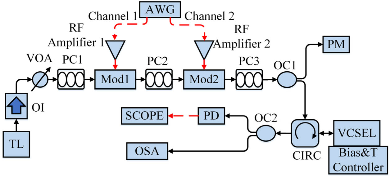
Fig. 1. Experimental setup of the binary convolution system based on a single VCSEL. TL, tunable laser; OI, optical isolator; VOA, variable optical attenuator; PC1, PC2, and PC3, polarization controllers; AWG, arbitrary waveform generator; Mod1, Mod2, Mach–Zehnder modulators; OC1, OC2, optical couplers; CIRC, circulator; Bias & T Controller, bias and temperature controller; PD, photodetector; PM, power meter; SCOPE, oscilloscope; OSA, optical spectrum analyzer.
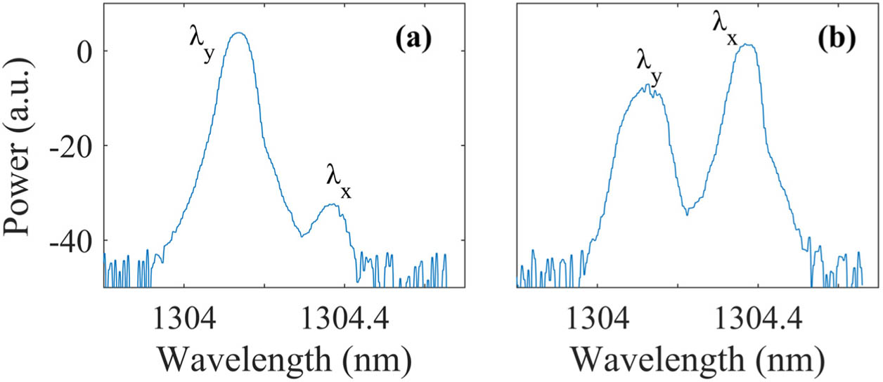
Fig. 2. (a) Optical spectrum of free-running VCSEL used in the experiment. (b) Optical spectrum of the VCSEL subject to constant optical injection. Two polarization modes of VCSELs are referred to as λ y λ x
Fig. 3. Example of a single step during a 2D binary convolution operation. During this step, a Hadamard (element-wise) product is calculated for a submatrix of the image and the kernel, and all of the values in the multiplication result are summed up to obtain a single value.
Fig. 4. Experimental convolution operation. (a) Inputs of Channel 1 (image in Fig. 3 ). (b) Inputs of Channel 2 (kernel in Fig. 3 ). (c) Inputs of VCSEL. (d) Outputs of VCSEL (the results of convolution).
Fig. 5. Temporal map of 100 superimposed consecutive convolutional results measured experimentally at the output of spiking VCSEL neuron.
Fig. 6. (a) Gray color: range of the local binary pattern descriptor of pixels. (b) A 24 × 24 B X + B X − B Y + B Y − 5 × 5
Fig. 7. Four convolutional results with four highlighted area kernels for one pixel, which has red box in Fig. 6 .
Fig. 8. Gradient maps of the “Square” source image. Visualizations of (a) G G X G Y
Fig. 9. “Horse head” image and the gradient maps of the “Horse head” image. (a) Source “Horse” image. The blue box indicates the “Horse Head” image used for analysis in (b). Visualizations of the (c) G G X G Y
Fig. 10. (a1)–(a3) Inputs of Channel 1 (image in Fig. 3 ). (b1)–(b3) Inputs of Channel 2 (kernel in Fig. 3 ). (c1)–(c3) VCSEL neuron’s output. (a1)–(c1) Convolutional operation in the VCSEL neuron without noise. (a2)–(c2) Convolutional operation in the VCSEL neuron with added input noise of SNR = 20 dB 5 × 5
Fig. 11. “Horse” image and gradient maps of the “Horse” image. (a) “Horse” image. Visualizations of (b) G G X G Y

Set citation alerts for the article
Please enter your email address
© Copyright 2018-2021 | Chinese Laser Press. All Rights Reserved 沪ICP备15018463号-20